
A. M. Y. Razak Thesis 1984
182
CRANFIELD NSTITUTEOF TECHNOLOGY SCHOOL F MECHANICAL NGINEERING PhD Thesis A. M. Y. RAZAK Dynamic Simulation of Centrifugal Compressors in a Process Environment Supervisor: Dr. R. L. Elder October 1984
Transcript of A. M. Y. Razak Thesis 1984
8/6/2019 A. M. Y. Razak Thesis 1984
http://slidepdf.com/reader/full/a-m-y-razak-thesis-1984 1/181
CRANFIELDNSTITUTEOF TECHNOLOGY
SCHOOL F MECHANICALNGINEERING
PhD Thesis
A.M.Y. RAZAK
Dynamic Simulation of Centrifugal
Compressors in a Process Environment
Supervisor: Dr. R. L. Elder
October 1984

8/6/2019 A. M. Y. Razak Thesis 1984
http://slidepdf.com/reader/full/a-m-y-razak-thesis-1984 2/181
To My Mother I Dedicate This Work
8/6/2019 A. M. Y. Razak Thesis 1984
http://slidepdf.com/reader/full/a-m-y-razak-thesis-1984 3/181
SUMMARY
The recent developments in process plant design have made it
desirable that a better understanding of transient compressor performance
within the process plant be gained. The model outlined in this thesis is
capable of representing most types of process plants. Further the
number of degress of freedom, plus the dynamic flexibility of a poly-
tropic analysis allow any system transient to be simulated, including
compressor surge. A computer program has been developed from the
model and validated using a small centrifugal compressor. The results
showing successful simulation of compressor transient behaviour
(including surge) are given. The model was then applied to study
the transient behaviour of a natural Gas Transmission station. The
model successfully highlighted compressor surge problems under certain
operative conditions. This surge phenomenons present in the trans-
mission station and a possible solution to the problem was suggesteddue to the better understanding of dynamic response of station.

8/6/2019 A. M. Y. Razak Thesis 1984
http://slidepdf.com/reader/full/a-m-y-razak-thesis-1984 4/181
ACKNOWLEDGEMENTS
The author would like to thank the various membersof the
School of Mechanical Engineering at Cranfield Institute of Technology
who have given help and advice during this project. In particular
Dr. R. L. Elder and Mrs. M.E. Gill for their advice and Mr. C. J. Austin
of British Gas Corporation for releasing the necessary information
for use in this project, and for their continuing interest.
8/6/2019 A. M. Y. Razak Thesis 1984
http://slidepdf.com/reader/full/a-m-y-razak-thesis-1984 5/181
CONTENTS
1.0 Introduction.... .... .... .... .... ..
I
2.0 The Mathematical Model 4
2.1 Derivation of the Basic Dynamic Equation 5
2.2 Continuity Equation 5
2.3 MomentumEquation 6
2.4 Lumpedand Linearly Distributed Parameter 7
2.5 LumpedParameter Model 7
2.6 Linearly Distributed Parameter Model 72.7 Choice of Model 8
2.8 Dynamics of the Energy Equation 8
2.9 ThermodynamicRelationships to Account for Real Gases 9
2.10 Calculation of Element Variables 10
2.11 Branch Elements (Flows Combining and Dividing) 12
2.12 Conclusions 13
3.0 Application of the Model 14
3.1 Frequency Parameter Model 14
3.2 Equalised Model 15
3.3 Definition of Element Types 15
3.4 Compressor Element - 16
3.5 Duct with Loss Element 17
3.6 Diffusing or Contracting Element .... .... ....18
3.7 Curved Duct Element 183.8 Recycle Valve Element 19
3.9 Branching Element 19
3.10 Blow Off Valve Element 20
3.11 Non-Return Valve Element 21
3.12 Boundary Conditions 22
3.13 Impedance ("near infinite volume") Boundary Condition 22
3.14 Nozzle Boundary Condition 23
3.15 Butt Boundary Condition 23
3.16 Conclusions 23
8/6/2019 A. M. Y. Razak Thesis 1984
http://slidepdf.com/reader/full/a-m-y-razak-thesis-1984 6/181
4.0 Review of Numerical Methods 25
4.1 Taylor-Series Method 25
4.2 Euler and Modified Euler Method 26
4.2.1 Euler Method 264.2.2 Modified Euler Method 27
4.3 Runge-Kutta Second Order Method 28
4.4 Runge-Kutta Fourth Order Method 28
4.5 Runge-Kutta-Merson Method 29
4.6 Runge-Kutta-Felberg Method 30
4.7 Multi-Step Method 31
4.8 Adams Method 31
4.9 Milner Method 32
4.10 Adams-MouldonMethod 32
4.11 Hamming's Method 33
4.12 Gear's Method 34
4.13 Conclusions 35
5.0 Experimental Validation of Mathematical Model 36
5.1 Description of Test Rig and Instrumentation 36
5.2 Compressor Test 37
5.3 Compressor Transient Between Stable Points 37
5.4 Surge Tests 37
5.5 Data Analysis 38
5.6 Simulation of Compressor Transients 39
5.7 Setting up of Data for Simulation .... .... ..39
5.8 The Simulation Program TRANS41
5.9 Program Performance 42
5.10 The Simulation of Measured Transients 44
5.11 Comparison of Measured and Simulated Transients 45
5.12 Conclusions 46
6.0.
Application of the Model to Simulate the Dynamic Response of
the Gas Transmission Station 48
6.1 Further Development of Program 48
6.2 Patching Procedure 48
6.3 Patching Procedure for the Gas Transmission Station 49
6.4 System Boundary Conditions 50
8/6/2019 A. M. Y. Razak Thesis 1984
http://slidepdf.com/reader/full/a-m-y-razak-thesis-1984 7/181
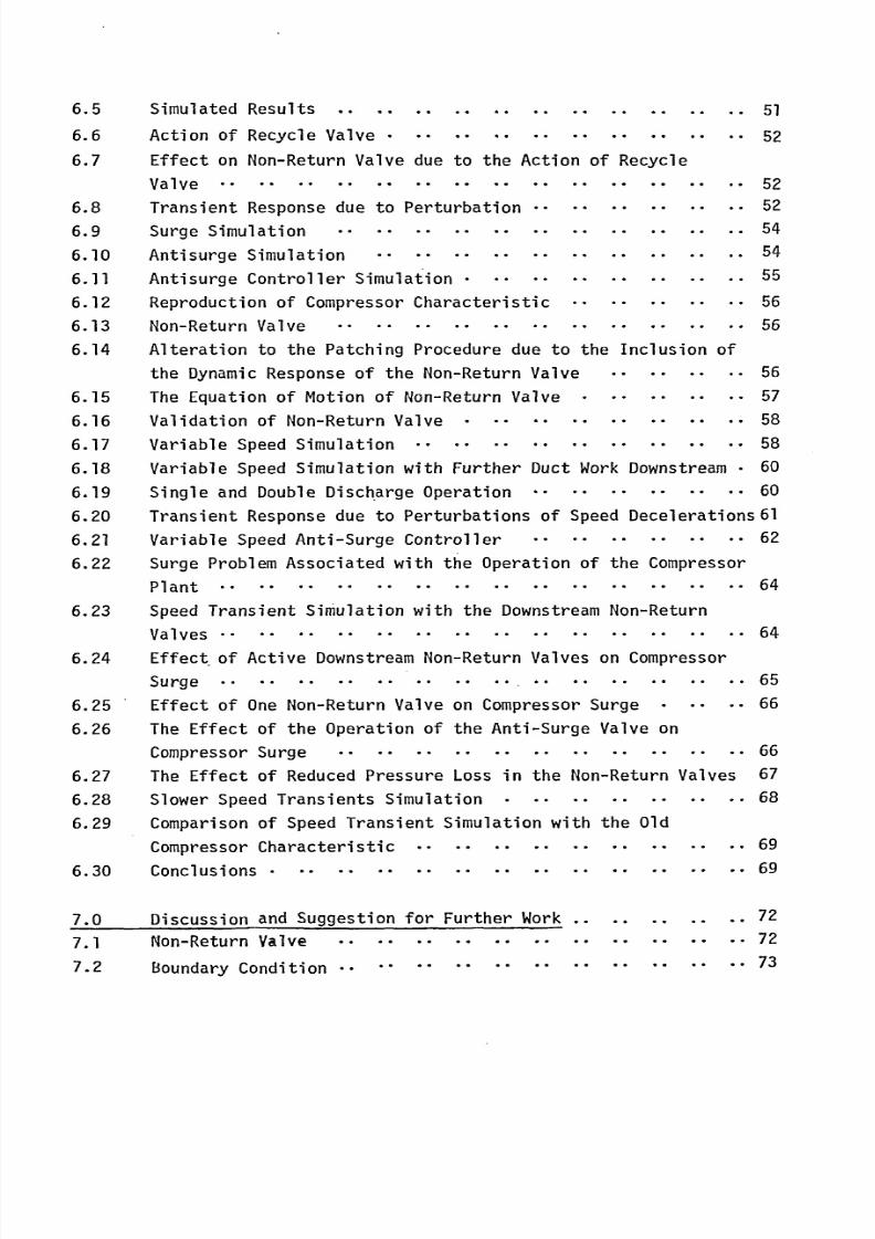
6.5 Simulated Results 51
6.6 Action of Recycle Valve 52
6.7 Effecton
Non-Return Valve due to the Actionof
Recycle
Valve 52
6.8 Transient Response due to Perturbation 52
6.9 Surge Simulation 54
6.10 Antisurge Simulation 54
6.11 Antisurge Controller Simulation 55
6.12 Reproduction of Compressor Characteristic 56
6.13 Non-Return Valve 56
6.14 Alteration to the Patching Procedure due to the Inclusion of
the Dynamic Response of the Non-Return Valve 56
6.15 The Equation of Motion of Non-Return Valve 57
6.16 Validation of Non-Return Valve 58
6.17 Variable Speed Simulation 58
6.18 Variable Speed Simulation with Further Duct Work Downstream 60
6.19 Single and Double Disch.arge Operation 60
6.20 Transient Response due to Perturbations of Speed Decelerations6l6.21 Variable Speed Anti-Surge Controller 62
6.22 Surge Problem Associated with the Operation of the Compressor
Plant 64
6.23 Speed Transient Simulation with the DownstreamNon-Return
Valves 64
6.24 Effect. of Active DownstreamNon-Return Valves on Compressor
Surge 65
6.25 Effect of One Non-Return Valve on Compressor Surge 66
6.26 The Effect of the Operation of the Anti-Surge Valve on
Compressor Surge 66
6.27 The Effect of Reduced Pressure Loss in the Non-Return Valves 67
6.28 Slower Speed Transients Simulation 68
6.29 Comparison of Speed Transient Simulation with the Old
Compressor Characteristic 69
6.30 Conclusions 69
7.0 Discussion and Suggestion for Further Work 72
7.1 Non-Return Valve 72
7.2 Boundary Condition 73
8/6/2019 A. M. Y. Razak Thesis 1984
http://slidepdf.com/reader/full/a-m-y-razak-thesis-1984 8/181
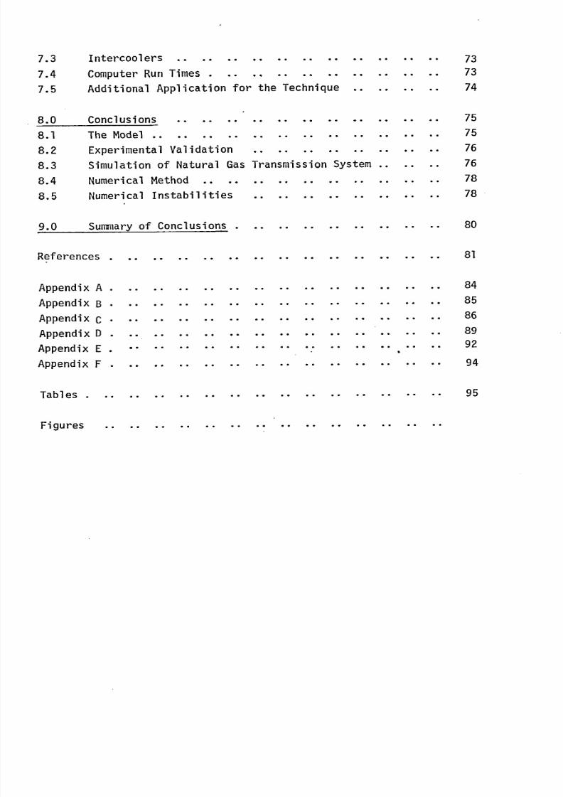
7.3 Intercoolers 73
7.4 Computer Run Times 73
7.5 Additional Application for the Technique 74
8.0 Conclusions 75
8.1 The Model 75
8.2 Experimental Validation 76
8.3 Simulation of Natural Gas Transmission System 76
8.4 Numerical Method 78
8.5 Numerical Instabilities 78
9.0 Summaryof Conclusions 80
References 81
Appendix A- 84
Appendix B- 85
Appendix C.86
Appendix D- 89Appendix E
92
Appendix F 94
Tabl es 95
Figures
8/6/2019 A. M. Y. Razak Thesis 1984
http://slidepdf.com/reader/full/a-m-y-razak-thesis-1984 9/181
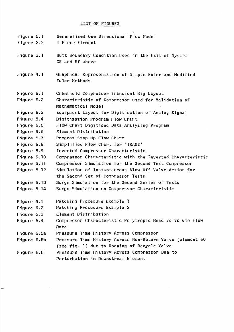
LIST OF FIGURES
Figure 2.1
Figure 2.2
Figure 3.1
Figure 4.1
Figure 5.1
Figure 5.2
Figure 5.3
Figure 5.4
Figure 5.5
Figure 5.6
Figure 5.7Figure 5.8
Figure 5.9
Figure 5.10
Figure 5.11
Figure 5.12
Figure 5.13
Figure 5.14
Figure 6.1
Figure 6.2
Figure 6.3
Figure 6.4
Figure 6.5a
Figure 6.5b
Figure 6.6
Generalised One Dimensional Flow Model
T Piece Element
Butt Boundary Condition used in the Exit of System
CE and Bf above
Graphical Representation of Simple Euler and Modified
Euler Methods
Cranfield Compressor Transient Rig Layout
Characteristic of Compressor used for Validation of
Mathematical Model
Equipment Layout for Digitisation of Analog Signal
Digitisation Program Flow Chart
Flow Chart Digitised Data Analysing Program
Element Distribution
Program Step Up Flow ChartSimplified Flow Chart for 'TRANS'
Inverted Compressor Characteristic
Compressor Characteristic with the Inverted Characteristic
Compressor Simulation for the Second Test Compressor
Simulation of Instantaneous Blow Off Valve Action for
the Second Set of Compressor Tests
Surge Simulation for the Second Series of Tests
Surge Simulation on Compressor Characteristic
Patching Procedure Example I
Patching Procedure Example 2
Element Distribution
Compressor Characteristic Polytropic Head vs Volume Flow
Rate
Pressure Time History Across CompressorPressure Time History Across Non-Return Valve (element 60
(see fig. 1) due to Opening of Recycle Valve
Pressure Time History Across Compressor Due to
Perturbation in DownstreamElement
8/6/2019 A. M. Y. Razak Thesis 1984
http://slidepdf.com/reader/full/a-m-y-razak-thesis-1984 10/181
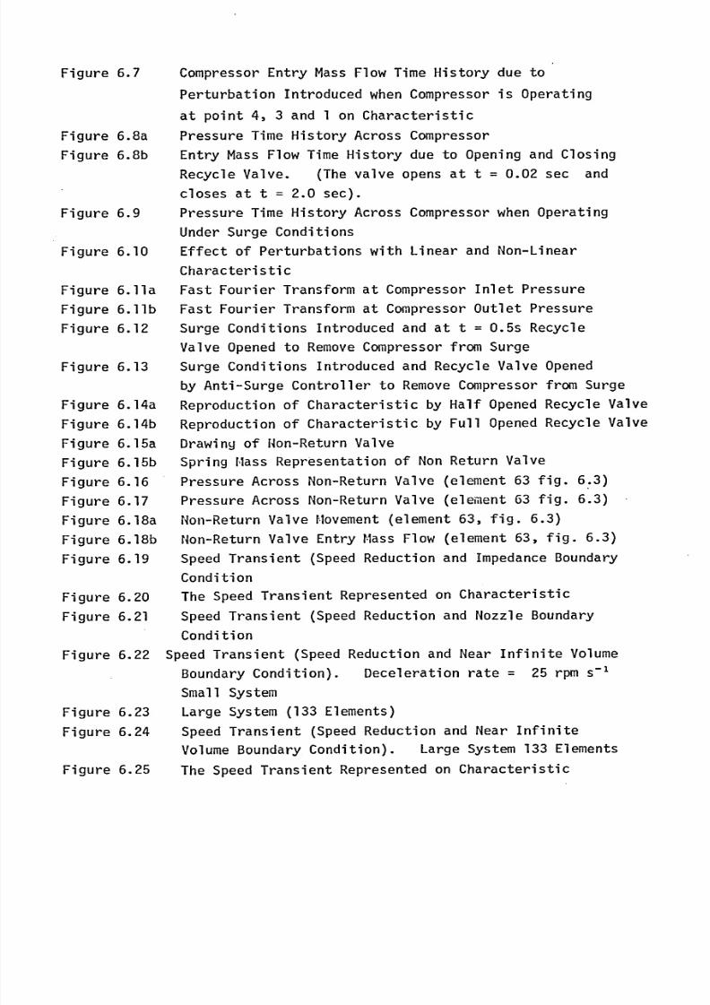
Figure 6.7
Figure 6.8aFigure 6.8b
Figure 6.9
Figure 6.10
Figure 6.11a
Figure 6.11b
Figure 6.12
Figure 6.13
Figure 6.14a
Figure 6.14b
Figure 6.15a
Figure 6.15b
Figure 6.16
Figure 6.17
Figure 6.18a
Figure 6.18b
Figure 6.19
Figure 6.20
Figure 6.21
Compressor Entry Mass Flow Time History due to
Perturbation Introduced when Compressor is Operating
at point 4,3 and 1 on Characteristic
Pressure Time History Across CompressorEntry Mass Flow Time History due to Opening and Closing
Recycle Valve. (The valve opens at t=0.02 sec and
closes at t=2.0 sec).
Pressure Time History Across Compressor when Operating
Under Surge Conditions
Effect of Perturbations with Linear and Non-Linear
Characteristic
Fast Fourier Transform at Compressor Inlet Pressure
Fast Fourier Transform at Compressor Outlet Pressure
Surge Conditions Introduced and at t=0.5s Recycle
Valve Opened to RemoveCompressor from Surge
Surge Conditions Introduced and Recycle Valve Opened
by Anti-Surge Controller to RemoveCompressor from Surge
Reproduction of Characteristic by Half Opened Recycle Valve
Reproduction of Characteristic by Full Opened Recycle Valve
Drawing of Hon-Return Valve
Spring Mass Representation of Non Return Valve
Pressure Across Non-Return Valve (element 63 fig. 6.3)
Pressure Across Non-Return Valve (element 63 fig. 6.3)
Non-Return Valve flovement (element 63, fig. 6.3)
Non-Return Valve Entry Mass Flow (element 63, fig. 6.3)
Speed Transient (Speed Reduction and Impedance BoundaryCondition
The Speed Transient Represented on Characteristic
Speed Transient (Speed Reduction and Nozzle Boundary
Condition
Figure 6.22 Speed Transient (Speed Reduction and Near Infinite Volume
Figure 6.23
Figure 6.24
Figure 6.25
Boundary Condition). Deceleration rate = 25 rpm s-1
Small System
Large System (133 Elements)
Speed Transient (Speed Reduction and Near Infinite
Volume Boundary Condition). Large System 133 Elements
The Speed Transient Represented on Characteristic
8/6/2019 A. M. Y. Razak Thesis 1984
http://slidepdf.com/reader/full/a-m-y-razak-thesis-1984 11/181
Figure 6.26
Figure 6.27
Figure 6.28
Figure 6.29
Figure 6.30
Figure 6.31
Figure 6.32
Figure 6.33
Figure 6.34
Figure 6.35
Figure 6.36
Figure 6.37
Figure 6.38
Figure 6.39a
Figure 6.39b
Figure 6.40a
Figure 6.40b
Figure 6.41a
Figure 6.41b
Figure 6.42
Figure 6.43
Figure 6.44
Speed Transient with Single and Double Discharge Operation
Speed Transient Represented on Characteristic
Speed Transient with Single and Double Discharge Operation.
Deceleration = -250 rpm/secSpeed and Delayed Pulse Transients
Speed and Delayed Throttling of DownstreamFlow Transient
Speed and Controller Actuation of Recycle Valve. Late
Opening of Recycle Valve
Speed & Delayed Pulse Transient Represented on Characteristic
Speed and Controller Actuation of Recycle Valve. Early
Opening
Speed Transient with both Downstream Discharge Line
Non-Return Valves in place
Speed Transient and Pressure Transient. The Pressure
Transient causes the last non-return valve in the discharge
line to closeNon-Return Valve (1) Movement due to Pressure and Speed
Transient
Non-Return Valve (2) Movementdue to Pressure and Speed
Transient
Non-Return Valve (1) Pressure Difference Time History due
to Speed and Pressure Transient
Non-Return Valve (2) Pressure Difference Time History due
to Speed and Pressure Transient
Mass Flow Rate Through Non-Return Valve (1) Time History
due to Speed and Pressure Transient
Mass Flow Rate Through Non-Return Valve (2) Time History
due to Speed and Pressure Transient
Non-Return Valve (3) Pressure Difference Time History due
to Speed and Pressure Transient
Speed and Delayed Pressure Transient. The Delayed
Pressure Transient Closes Non-Return Valve (1)
Speed and Pressure Transient with Non-Return Valves
(2) and (3)
8/6/2019 A. M. Y. Razak Thesis 1984
http://slidepdf.com/reader/full/a-m-y-razak-thesis-1984 12/181
Figure 6.45
Figure 6.46
Figure 6.47a
Figure 6.47b
Figure 6.48
Figure 6.49
Figure 6.50a
Figure 6.50b
Figure 6.51
Figure 6.52
Figure 6.53
Speed Transient and the Opening of Recycle Valve to
Avoid Surge Conditions
Speed Transient with Reduced Pressure Loss in Non-
Return Valves
Non-Return Valve (1) Movementdue to Speed Transient
with Reduced Pressure Loss in Non-Return Valves
Non-Return Valve (2) Movementdue to Speed Transient
with Reduced Pressure Loss in Non-Return Valves
Speed Transient (deceleration rate = 25 rpm sec-'
with no DownstreamNon-Return Valves
Speed Transient (deceleration rate = 25 rpm sec-'
with Reduced Pressure Loss in Non-Return Valve
Non-Return Valve (1) Movementdue to Reduced Pressure
Loss in Non-Return Valves. (Deceleration = 25 rpm sec-1)Non-Return Valve (2) Movementdue to Reduced Pressure
Loss in Non-Return Valves. (Deceleration = 25 rmp sec-1)
Slow Speed Transient with reduced pressure loss in Non-Return
Valve, Represented on Characteristic
Speed Transient with Steep Compressor Characteristic andReduced Pressure Loss in Hon-Return Valves
Proposed Layout of Transmission Station
8/6/2019 A. M. Y. Razak Thesis 1984
http://slidepdf.com/reader/full/a-m-y-razak-thesis-1984 13/181
NOTATION
Area (M2)
Cp Specific Heat at Constant Pressure (J/kgK)
Cv Specific Heat at Constant Volume (J/kgK)
c Velocity (m/s)
d Diameter (m)
e Polytropic Effic. iency H
E Energy P)
Enet
Net Input of Energy into an Element P)
f Pipe Resistance Coefficient
fp Polytropic Head Factor
F Body Force
Fnet Net Body Force Acting Within an Element
h Integration Time-Step Length
H Stagnation Enthalpy
KE Kinetic Energy
Ks Static Pressure Coefficient
L Length
HH(Pa)
(Pa)
(S)(J/kg)
P)H
(m)
M Schultz Polytropic Index H
M Mach Number H
MW Molecular Weight (kg)
n Polytropic Index
N Compressor Shaft Speed
Pt Stagnation Pressure
PS Static Pressure
(r. p. m.
(pa)
(Pa)
8/6/2019 A. M. Y. Razak Thesis 1984
http://slidepdf.com/reader/full/a-m-y-razak-thesis-1984 14/181
Volumetric FlowRate(M3 /hr)
R Gas Constant
Re Reynold's Number
S Surface Area
S Compressor Speed
(J/kgK)
H
(M2)
(m/sec)
t Time (s)
Tt Stagnation Temperature (K)
TsStatic Temperature (K)
U Pipe Resistance Function
v Volume
W Mass Flow
Wp Polytropic Head
WS Shaftwork
x Axial Direction
X Compressibility Function
z
Pipe Resistance Function
Compressibility Function
Compressibility Factor
(- )
(me)
(kg/s)
(J/kg)
(J/kg)
HH
HH
C-.
Ax Element Length (m)
F- Surface Roughness (m)
Y Ratio of Specific Heats H
P Stagnation Density (kg/m')
8/6/2019 A. M. Y. Razak Thesis 1984
http://slidepdf.com/reader/full/a-m-y-razak-thesis-1984 15/181
I
CHAPTER
1.0 INTRODUCTION
Until recently, relatively little attention has been paid to -
the prediction of transient behaviour of dynamic compressors, and the
response rate of such compressors was established empirically during
testing. Now, however, the transient behaviour is often predicted by
mathematical models and a detailed knowledge of the dynamic response
at the design stage is becoming increasingly important for the design
and development of control systems. This is particularly the case in
the aero gas turbine industry where it is commonpractice for manufacturers
to be asked to guarantee the transient behaviour of their products
when negotiating contracts.
A full analytical model considering all the aerodynamic factorsare considered not practical, and much simplified one dimensional models
based on the conservation of linear momentum nd continuity have been
developed for aero space industry. In spite of the limitations such
a model has (i. e. element length) very promising results have been
obtained. The steady state compressor characteristics have been used
to introduce effects of the blading or impeller depending on the type
of compressor being considered. (I. e. axial or centrifugal).
This trend has now been reflected in the process plant industry
where the transients may be introduced by the operation of many process
plant controls and/or the change in gas composition. Within such
industry the use of large centrifugal compressors. in application such as
the compression of process gas, and especially natural gas transmission,
is wide spread. Unlike the steady state performance of these machines
the transient response are, as yet, little understood. Still lesswell understood is the interaction of these machines with plant controls
during rapid transients such as compressor surge, sudden start up/shut
down, and sudden operation of valves. Therefore the design of control
systems to govern the behaviour of the plant during such transient
8/6/2019 A. M. Y. Razak Thesis 1984
http://slidepdf.com/reader/full/a-m-y-razak-thesis-1984 16/181
2
operation is difficult, and in many cases results in inefficient design
due to, on the one hand, over specification, and on the other, under
estimation which can lead to catastropic failure of critical plant
components leading to high operation cost and/or repair.
The development of such computer models for the process industry
must be more general and therefore such models should have the capability
of simulating compressors operating in parallel and precise modelling
of plant controls where transients are likely to be introduced. The
transient effect due to change in gas composition must also be a feature.
Further to this the model must have the ability of simulating compressor
surge and have sufficient thermodynamic flexibility in order that various
gases, that are commonly used in process industry, may be represented.
To gain this much needed understanding of the installed dynamic
response of the compressor a research program was carried out involving
British Gas Corporation and ICI Agricultural Division Ltd., which
developed a mathematical model capable of simulating compressor transient
performance, including compressor surge within the process environment.The model was originally developed for an aero-space application, and
has been extensively modified for an industrial user where the working
fluid need not necessarily be air. In addition to this transient data
has been acquired using a small high speed centrifugal compressor (of
a turbo-charger) for model validation purposes.
Theavailability of such models also enable
thesimulation of
existing process plants where the plant may have suffered from compressor
instabilities in the past, particularly those plants where a satisfactory
solution to the instability problem was not found. Further to this,
when plant modifications are planned the simulation of the transient
response of the proposed system may highlight operational problems and
remedies may be found at the planning stage. Whencompressor in-
stabilities result in plant failure the model may be used to investigate
the cause of failure.
The model was applied to study the dynamic response of a
British Gas transmission station. The plant was selected as an
8/6/2019 A. M. Y. Razak Thesis 1984
http://slidepdf.com/reader/full/a-m-y-razak-thesis-1984 17/181
8/6/2019 A. M. Y. Razak Thesis 1984
http://slidepdf.com/reader/full/a-m-y-razak-thesis-1984 18/181
4
CHAPTER
2.0 THE MATHEMATICALODEL
The successful simulation of compressor transients requires
that the model used must have sufficient flexibility to simulate
compressor surge and the ability to represent non-ideal gases. The
wide availability of steady state compressor characteristics describing
compressor performance between upstream and downstream stations
suggests the use of such data in any model. This also suggests the
use of a one dimensional model neglecting the detailed modelling of
secondary flow, rotating stall and other related three dimensional
phenomenon.
.Numerouscompressor models have been developed to study the transient
behaviour of industrial compressors although none (Ref. 1-6) have the
capability of simulating compressor surge. Faso] Ref. (5,6), however,
has produced good results when simulating rapid transfers between
stable compressor operator points and applies the model to a blast
furnaceplant where the flow may branch into other systems. In this
respect the system considered there is similar, (to the problem consid-
ered inthis thesis), but theability to.combine flowsas in recycle loops
was not considered(a feature
availablein the proposed model). The
applicability of the techniques proposedin thisthesis areconsidered tobe
more general than those of Fasol and the capability of simulating
compressor surge is an added feature of the proposed model.
To achieve a concise model the flow has been assumedto be one
dimensional. The transient basis of the model is achieved by
considering the conservation relations in their dynamic form.
Models of this type have been proposed previously, for instance the
work of Kulberg et al (7 ), Willoh and Seldner (8), and Elder (9,10,11)
suggests models which are capable of simulating compressor surge and
Greitzer (12) has used similar models to that proposed here to simulate
8/6/2019 A. M. Y. Razak Thesis 1984
http://slidepdf.com/reader/full/a-m-y-razak-thesis-1984 19/181
5
post stall behaviour of compressors. These models, however, did not
consider parallel flow path systems such as those described here.
The thermodynamic flexibility to model non-ideal gases has been
much less generally considered although Davis (1) (in a simple dynamic
model) used the quite powerful Bendict-Webb-Rubin equation of state.
A more manageable method, however, is presented by Schultz (13), and
is employed in the proposed model. The compressibility charts x, y
and z referred to by Schultz are plotted in terms of reduced pressures
and reduced temperatures. These charts are very much the samefor
all gases, therefore making it much easer to use.
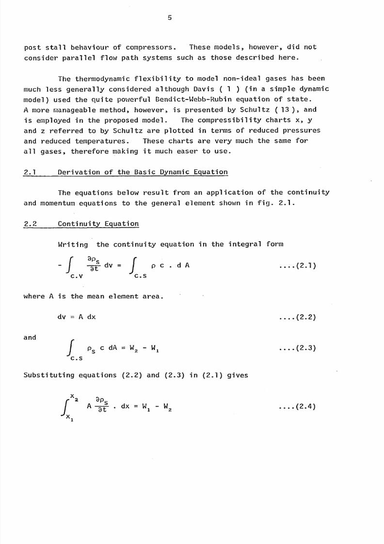
2.1 Derivation of the Basic Dynamic Equation
The equations below result from an application of the continuity
and momentum quations to the general element shown in fig. 2.1.
2.2_Continu-ity
Equation
Writing the continuity equation in the integral form
-
ýpsdv =1pc. dA
DtC. V C. S
where A is the meanelement area.
dv =A dx....
(2.2)
and
c dA =W2-wI (2.3)
C. S
Substituting equations (2.2) and (2.3) in (2.1) gives
xADps
.dx
f
Dt
xl
(2.4)
8/6/2019 A. M. Y. Razak Thesis 1984
http://slidepdf.com/reader/full/a-m-y-razak-thesis-1984 20/181
6
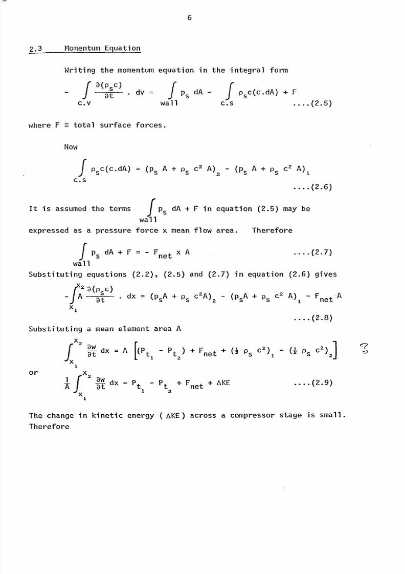
2.3 MomentumEquation
Writing the momentum quation in the integral form
f
atdv =fps dA -f PS (c. dA) +F
C.v wall C.S ....(2.5)
where F =- total surface forces.
Now
PS (c. dA) = (psA+pSc2
A)2-
(PS A+pSc2 A)1
C. S
....(2.6)
It is assumedthe termsf
ps A+F in equation (2.5) may be
wall
expressed as a pressure force x meanflow area. Therefore
fpsdA +FF
netxA.... (2.7)
wall
Substituting equations (2.2), (2.5) and (2.7) in equation (2.6) gives
dx = (p A+p OA) (p A+pc2 A) FA
2
ssss netR
1
(2.8)
Substituting a mean element area A
or
2)-wdx =Ap Pt )+F2pcI
at
1(
tI-2 net+ (I Ps Cs2
x2
f
atdx = Pt
....(2.9)- Pt + Fnet + AKE
-.
T12
x
x1
x
1
The change in kinetic energy ( AKE) across a compressor stage is small.
Therefore
8/6/2019 A. M. Y. Razak Thesis 1984
http://slidepdf.com/reader/full/a-m-y-razak-thesis-1984 21/181
7
xf2 aw
dx =PTt- ti - Pt2+
Fnet
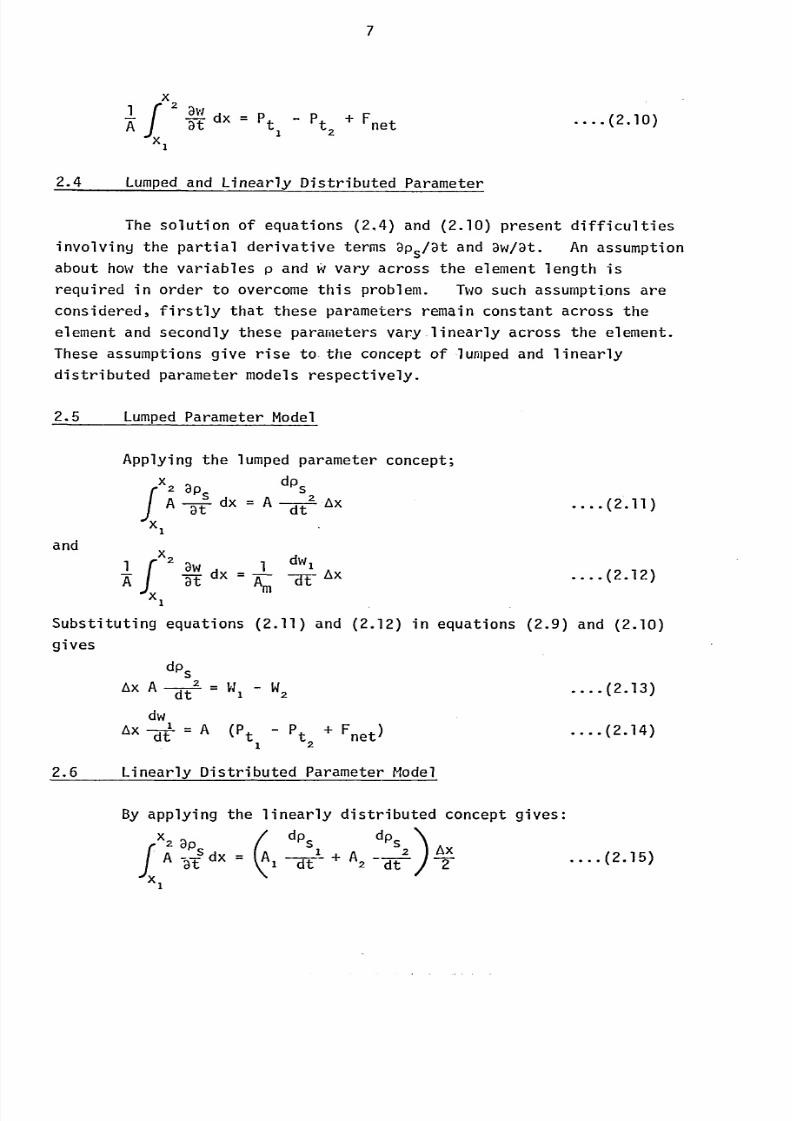
2.4 Lumpedand Linearly Distributed Parameter
Applying the lumped parameter concept;
x2 3Ps
dps2AX
A -5-t dx =A dt
The solution of equations (2.4) and (2-10) present difficulties
involving the partial derivative terms Dp, Dt and 3w/3t. An assumption
about how the variables p and Wvary across the element length is
required in order to overcome this problem. Two such assumptions are
considered, firstly that these parameters remain constant across the
element and secondly these parameters vary linearly across the element.
These assumptions give rise to the concept of lumped and linearly
distributed parameter models respectively.
2.5 Lumped Parameter Model
and
xl
xl
fX2 , dw,3w dx = -a-t AxTt A
mxl
Substituting equations (2.11) and (2.12) in equations (2.9) and (2.10)gives
dps
Ax Adt
2=WI-w2
dwAx '=A (P-a-t tpt2+F
net)
(2.10)
2.11)
(2.12)
(2.13)
(2.14)
2.6 Linearly Distributed Parameter Model
By applying the linearly distributed concept gives:
x2 3pdp
sIdp
s2 AxA-ý tsdx=
(A
I- -a t- +A2 -dt
)-2
x
8/6/2019 A. M. Y. Razak Thesis 1984
http://slidepdf.com/reader/full/a-m-y-razak-thesis-1984 22/181
8
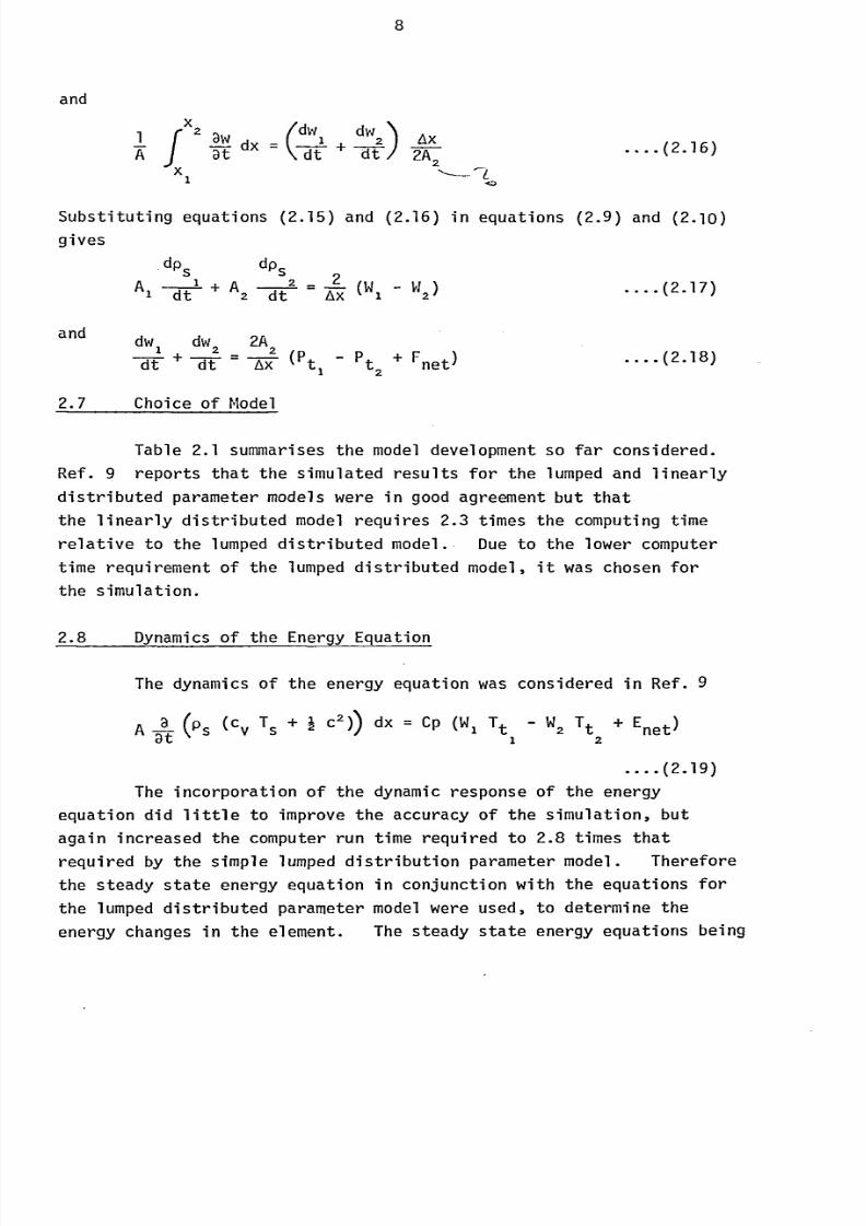
andx2
3ý1dx =dw
1+dw
2 AxTt
(
-dt -a-t) 2A2x
f
....(2.16)
Substituting equations (2.15) and (2.16) in equations (2.9) and (2.10)
gives
.dp
sdps
2A1+A2 (W w1 dt 2 dt
'Ä -x 12
and
2.7
dw,+
dw2 2A2-af -a-t :, -yx-
ptpt2+F
net)
Choice of Model
(2.17)
(2.18)
Table 2.1 summarises the model development so far considered.Ref. 9 reports that the simulated results for the lumped and linearly
distributed parameter models were in good agreement but that
the linearly distributed model requires 2.3 times the computing time
relative to the lumped distributed model.. Due to the lower computertime requirement of the lumped distributed model, it was chosen for
the simulation.
2.8 Dynamics of the Energy Equation
The dynamics of the energy equation was considered in Ref. 9
+1 C2)A -L
(P, (cvTs2
dx = Cp (Wl Tt W2 Tt +Enet)t 2
....(2.19)
The incorporation of the dynamic response of the energy
equation did little to improve the accuracy of the simulation, but
again increased the computer run time required to 2.8 times that
required by the simple lumped distribution parameter model. Thereforethe steady state energy equation in conjunction with the equations for
the lumped distributed parameter model were used, to determine the
energy changes in the element. The steady state energy equations being
8/6/2019 A. M. Y. Razak Thesis 1984
http://slidepdf.com/reader/full/a-m-y-razak-thesis-1984 23/181
9
H+Enet
1 wi
orTT..
Enet
52-, i, cpwI
(2.20)
....(2.21)
2.9 Thermodynamic Relationships to Account for Real Gases
To keep computational requirements down to a reasonable level
while retaining good accuracy under normal process plant operations the
Schultz method was used (Ref. 13), where the following compressibilityfactors are derived.
T (3Tv)p_Ia
P VýW)
T
(2.22)
(2.23)
These functions introduce effects to account for real gases in
the polytropic analysis given below. The equation of state used for
this model is the simple relationship:
PV = ZRT....
(2.24)
Schultz introduces a further term, fp- the polytropic head
factor, to take into account the difference between the true work and
the calculated work from the polytropic relationships discussed below.
Differences may occur when large change in state variables are present.
The analysis presented here neglects such refinements (fp = 1).
Since the state variable changes are relatively small, the following
equations are then obtained.
m=LR 1+Cp
(e
.
X)
WP=
Cp T, fpp2/Pl)
m-1)
G,X)((
(2.25)
(2.26)
8/6/2019 A. M. Y. Razak Thesis 1984
http://slidepdf.com/reader/full/a-m-y-razak-thesis-1984 24/181
10
WS=
ýE+ AKE
e
(P2
T2ýT,pl)
(2.27)
(2.28)
Using these equations allow the calculations of the steady
state outlet gas states given the inlet gas states and the gas properties
(Z, R, X, Cp), together with the compressor characteristic which will
usually define the polytropic head and efficiency as a function of
volume flow rate. This analysis is discussed further in the next
chapter where the Fnet and Enet terms are determined for a compressorelement.
2.10 Calculation of Element Variables
One further simplification is required for the chosen model
equations, which will overcome the need to calculate densities so that
theseequations may
determine theelement pressures
directly.
For an adiabatic process
PS
or
PS
PS k ps
where k =-constant
dps M-1
dpskmp
dt
dps
Psm dps
dt dts
PsSubstituting - ZRT
ps
dps dps-t ZRTm
dt
or dpsI
dps
....(2.29)
dt Z f-m -a Tt
8/6/2019 A. M. Y. Razak Thesis 1984
http://slidepdf.com/reader/full/a-m-y-razak-thesis-1984 25/181
11
Substituting in the model equation (2.4)
Ax Adp
S (w, wZRTM -Tt- 2)
dps
ZRTm
dt v
where V=A. Ax.
(2.30)
It is preferred to have total pressures and total temperatures
because compressor characteristics are expressed in termsof
totalsor
some function of totals (depending if the characteristic is represented
in pressure ratios or polytropic head).
Using:
pt+Y21M2) Yy
-ý S
andTt
+yIs
dPt
dps Y- 1 ,)
-Tt- ý -j12
Substituting in equation (2.30)
dPt= (W -+
'ý21
M2-d Tt 1
W2)v
(i-yY-1
includingTs
as a function Tt and m
dP ZRmTt(I
+ 17-1 m2)y
t= (W wv2dt 12+Y21 M2
or simplifying
dP ZRmT1
(W1-W2)Vt
(1+m2)
(2.31)
(2.32)
(2.33)
8/6/2019 A. M. Y. Razak Thesis 1984
http://slidepdf.com/reader/full/a-m-y-razak-thesis-1984 26/181
12
expanding
(I
+Y21 M2)y
using the binomial theorem
+ 1: 1 M2 +I M2 + _(2-y)(y-1) M4
228+ higher orders of m
Since it is assumed that m<0.3 then M2 ýU0. Therefore equation (2.33)
becomes
dPt
ZRmTt
--i-t -v (2.34)
Expressing the model equations in terms of station numbers:
dPt
ZRmTt
dtv
dw
dt ( t1-pt2+Fnet)
2.11 Branch Elements (Flows Combining and Dividing)
(2.35)
(2.36)
Fig. 2.2 shows such elements. The branch flow, W39
is assumed
to be at right angles to the main flow and therefore the momentum f
these flows do not take part in the momentum nalysis. Writing the
integral form of the continuity equation
ý-P dv =pcdAf at
f
C.v C. S
In this case
(2.37)
f
pcdA = (pcA)1-
(pcA)2±
(pcA)3=WI-W2±W3
C. S ...(2.38)
where the positive sign is for flows combining and negative sign is forflows dividi. ng. W3 is the flow rate during combination or dividing
(fig. 2.2).
8/6/2019 A. M. Y. Razak Thesis 1984
http://slidepdf.com/reader/full/a-m-y-razak-thesis-1984 27/181
13
Assuming a mean area for the element and using the lumped
parameter model assumption equation (2-38) becomes
dps1
dt = AAx(WI
-W2 i WO
Expressing in terms of total pressures and temperatures as
discussed in section 2.11
dP2
MRZTt
vW2±W3)
(2.39)
The momentumequation for these types of elements are unalteredand equation (2.36) is used.
2.12 Conclusions
The generalised flow element has been developed for one-
dimensional flow and although the model will not cope with complex three
dimensional compressor flows this limitation does not prevent the model
being used to simulate such elements if the element boundaries are chosen
sufficiently far upstream and downstream of the compressor and relevant
body force terms are available. This requirements also tends to imply
that the low Mach number assumption (in the model derivation) is
satisfied since the Mach numbers at these stations are generally below
0.3.
The choice of the lumped parameter model which neglects thedynamics of the steady state energy equation was justified on the
basis of saving computational efforts and because the frequency
restrictions so implied did not present any problem. The terms which
still need to be defined are the force term, Fnet, and the energy
term Enet*
The following chapter discusses the evaluation of these
terms for a series of elements.
8/6/2019 A. M. Y. Razak Thesis 1984
http://slidepdf.com/reader/full/a-m-y-razak-thesis-1984 28/181
14
CHAPTER
3.0 APPLICATIONOFTHE MODEL
During this chapter both the restrictions imposed by such
assumptions and the techniques used to model the various items of a
process plant (i. e. compressor, valves, pipework, etc. ) will be considered.
Several assumptions have been made in the derivation of the
model equations. The internal compressor flows where the flow direction
is complex cannot be modelled, and therefore in modelling such elements
it is necessary to chose station points sufficiently upstream and down-
stream of the compressor. The assumptions of low Mach number, discussed
in chapter 2, hold true only if the element boundaries are chosen to
avoid high velocity regions. For instance this assumption does not
hold if the element boundaries are chosen at the compressor impeller,
but holds at boundaries sufficiently upstream and downstream of the
impeller, (say at the compressor inlet and outlet flanges). The
assumptions of the lumped parameter distribution to overcome the
difficulties of the integral terms,(fA
-LPdx andf-Lw
dx) inax at
chapter 2, impose frequency limitations. If a frequency (,v) and a
velocity (c) is considered then the basic wavelength (assuming c << a,
the velocity of sound) is X= a/v and it was assumedthat the elementlength Ax << X i. e. if the frequency was 1OHzand the velocity of sound
340 ms-1 then Ax << 34m.
It is assumed an element length of-3m (<< 34m) enables a
longitudinal wave to traverse the length of the element several times
during a transient, and therefore capable to simulation such long-
itudinal wave forms.
3.1 Frequency Parameter Model-,
To account for the frequency of pre-surge oscillations, a
certain geometrical distribution wasthought necessary. Too large
an element length for the compressor element results in an unrealistic
8/6/2019 A. M. Y. Razak Thesis 1984
http://slidepdf.com/reader/full/a-m-y-razak-thesis-1984 29/181
15
response of the compressor surge. Too short an element length gives
an unsatisfactory pre-surge compressor response.
Earlier work of Elder, Ref. (11) related a frequency parameter
to the phase change across an element in terms of an expected errorwhen comparing the lumped parameter model with the true solution to
the partial differential equations. For a reasonable error (less than
5%) this suggests that:
- WRZT2Tr x Ax < Ily RT - AP
27T x Ax <a- Vx
21T x Ax <a (1 - Mx)
(3.1)
(3.2)
(3.3)
where P and T are the mean pressures and temperatures for the element.
Theexpected frequency of interest, fx, is used in the inequality
(3.1) to determine the element length Ax. The Mach number, Mx, is
taken to be about 0.3 or less. This yields the suitable elementlength for the compressor. This compressor length should be less than
that imposed by the frequency limitation discussed in section 3.0.
3.2 Equalised Model
Although the above analysis improves simulated results it was
found that theelements
donot
"communicate" ina realistic manner
if
the volumes of adjacent elements were significantly different. In
order that these elements interact with each other in a realistic
manner, a criterion of approximately equal volumes is used, in con-
junction with the frequency parameter concept. This ensures that the
elements take proper account of events occuring upstream and downstream.
Furthermore if adjacent element volumes are significantly different
the numerical solutions to the model equations becomestiff.
3.3 Definition of Element Types
All the terms in the model equations
8/6/2019 A. M. Y. Razak Thesis 1984
http://slidepdf.com/reader/full/a-m-y-razak-thesis-1984 30/181
16
dP2
MZRT2
--a -t = -V(Wi
2)
dWlAm
dt = E-x (PI - P2 + Fnet)
HH+Enet
21w1
(3.4)
(3.5)
(3.6)
are calculable with the exception of the energy term, Enet , and the
force term Fnet
(Enet
represents the energy input into an element, and
Fnet' the force exerted by the element on the flow). The assumption
is made that the Enet and Fnet terms may be calculated using the
instantaneous steady state values for the entry element parameters(e. g. inlet mass flows, pressures and temperatures). Evaluation of
Fnet and Enet
terms for the different types of elements ocurring in a
process plant are considered below.
3.4 Compressor Element ( -T9p jý ýý,I)
In the case of the compressor element the force term (Fnet in
(3.5)) is obtained from the stored compressor characteristic which is
of the form
Wp=
To.obtain Fnet the characteristics are interpolated to give the poly-
tropic head (Wp) and the polytropic efficiency (e). These are used
in the polytropic relations
WpCp T,
pX)
[(
ly
where =ZR (l
+ X)C-P eý
(3.7)
(3.8)
and X is the Schultz factor which like the Z factor, represents the
real gases effects (also see Schultz, ref. (13).
Since the force term, Fnet' is defined as the pressure rise in
8/6/2019 A. M. Y. Razak Thesis 1984
http://slidepdf.com/reader/full/a-m-y-razak-thesis-1984 31/181
17
steady state for the instantaneous flow rates then the Fnet
term in
equation (2.36)for the compressor element is equated to
I/
mFnet = P2 - P, pe+11
11 G+
X)
1
11(3.9)
The shaft work Wsfor a given polytropic efficiency, e, is given as
ws =
yp
e(3.10)
Substituting VIs
in the energy equation (3.6) we have the compressor out--
let temperature.
wsTT+-
21 Cp
or TT+WP
21e. Cp
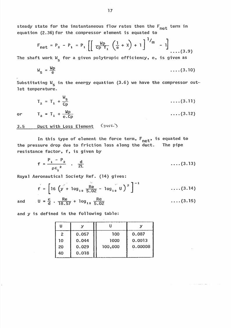
3.5 Duct with Loss Element (pW 1--)
....(3.11)
(3.12)
In this type of element the force term, Fnet'
is equated to
the pressure drop due to friction loss along the duct. The pipe
resistance factor, f, is given by
Ip
PC12
2L
Royal Aeronautical Society Ref. (14) gives:
16 + logloRe
- logl0U)2.02
and U= ýý Re+ loglo
Red* 18.57 5.02
and y is defined in the following table:
-1
u Y u y
2 0.057 100 0.087
10 0.044 1000 0.0013
20 0.029 100,000 0.00008
40 0.018
(3.13)
(3.14)
(3.15)
8/6/2019 A. M. Y. Razak Thesis 1984
http://slidepdf.com/reader/full/a-m-y-razak-thesis-1984 32/181
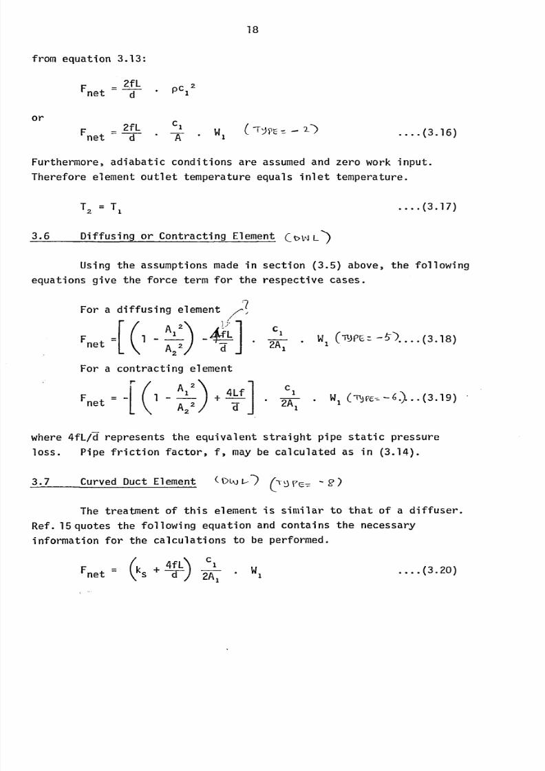
18
from equation 3.13:
or
2fL 2Fnet = ýd PCI
Fnet
2fL cl
dA7 ýVE ý-
.(3.16)
Furthermore, adiabatic conditions are assumedand zero work input.
Therefore element outlet temperature equals inlet temperature.
T2 :-T,
3.6 Diffusing or Contracting Element (OW L')
Using the assumptions made in section (3.5) above, the following
equations give the force term for the respective cases.
For a diffusing element
F1-A,
)
-4ý41 w ('R)pr--...
(3.18)net
I(A22
-j * 2A, I
For a contracting element
Fr
(1 A12)
+ 4Lf] Cl
Wnet : -
IA22
ýr * 2A, I
where 4fL/-d represents the equivalent straight pipe static pressure
loss. Pipe friction factor, f, may be calculated as in (3.14).
3.7 Curved Duct Element ( DLi I-) (vq VC, -2)
The treatment of this element is similar to that of a diffuser.
Ref. 15 quotes the following equation and contains the necessary
information for the calculations to be performed.
F(k 4f L) cl
.w....(3.20)
net s+a 2A, 1
8/6/2019 A. M. Y. Razak Thesis 1984
http://slidepdf.com/reader/full/a-m-y-razak-thesis-1984 33/181
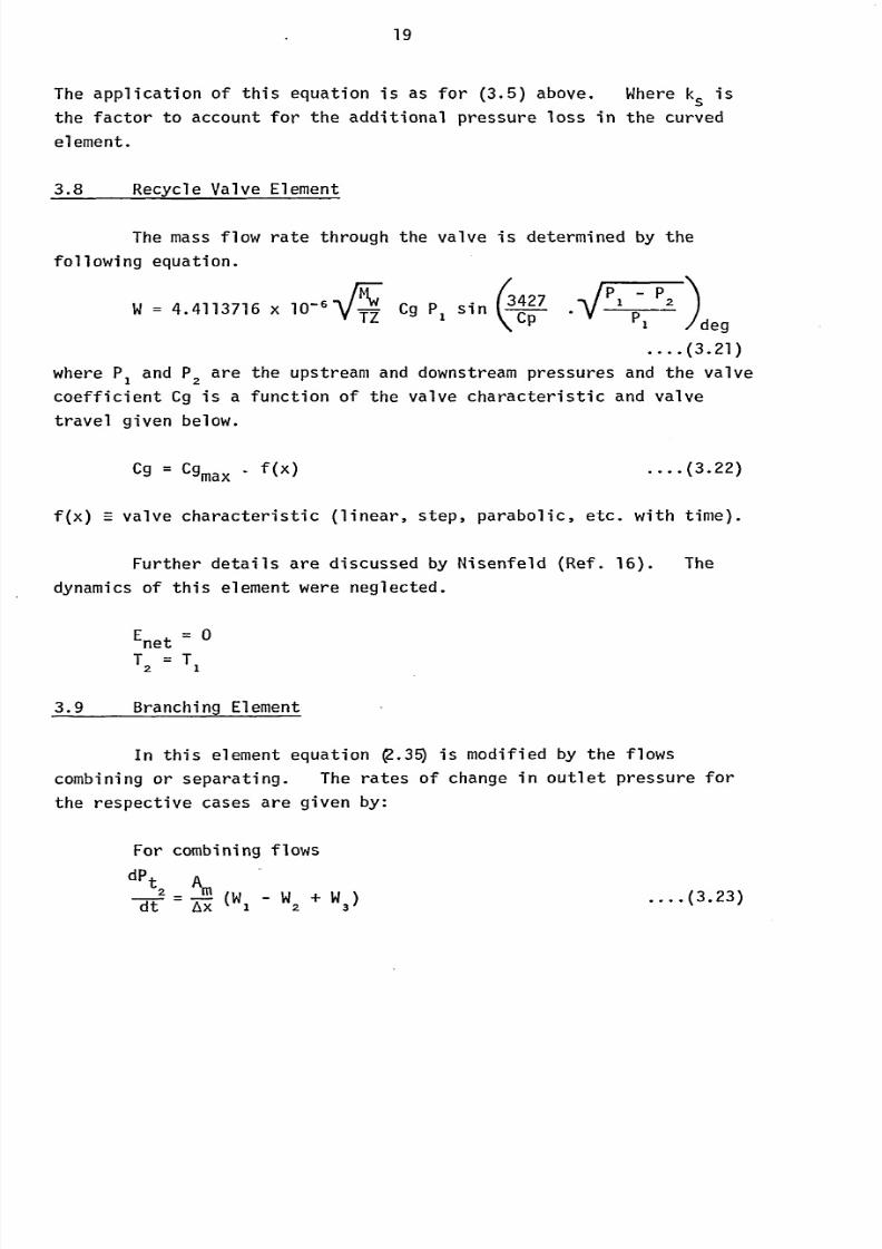
19
The application of this equation is as for (3.5) above. Where ks is
the factor to account for the additional pressure loss in the curved
element.
3.8 Recycle Valve Element
The mass flow rate through the valve is determined by the
following equation.
W=4.4113716 x 10-r"Fý Cg P, sin
(LC4-27
2pV
P1 ý2)deg
T-2 PI
.... (3.21)
where Pi and P2 are the upstream and downstream pressures and the valve
coefficient Cg is a function of the valve characteristic and valve
travel given below.
C9 = Cgmax'
f(x)....
(3.22)
a valve characteristic(linear,
step, parabolic, etc. withtime).
Further details are discussed by Nisenfeld (Ref. 16). The
dynamics of this element were neglected.
Enet
T2 :-T1
3.9 Branching Element
In this element equation ý. 3ý is modified by the flows
combining or separating. The rates of change in outlet pressure for
the respective cases are given by:
For combining flows
dPt? Am -
-=- (W -W+Wt Ax 123(3.23)
8/6/2019 A. M. Y. Razak Thesis 1984
http://slidepdf.com/reader/full/a-m-y-razak-thesis-1984 34/181
20
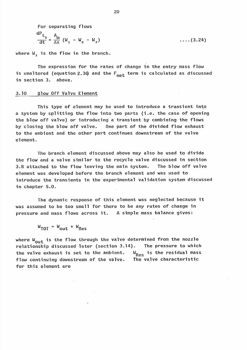
For separating flows
Ot
2A-= -T (W W-Wdt Ax 2
where W3 s the flow in the branch.
(3.24)
The expression for the rates of change in the entry mass flow
is unaltered (equation 2.3Q and the Fnet term is calculated as discussed
in section 3. above.
3.10 Blow Off Valve Element
This type of element may be used to introduce a transient inýo
a system by splitting the flow into two parts (i. e. the case of opening
the blow off valve) or introducing a transient by combining the flows
by closing the blow off valve. One part of the divided flow exhaust
to the ambient and the other part continues downstream of the valve
element.
The branch element discussed above may also be used to divide
the flow and a valve similar to the recycle valve discussed in section
3.8 attached to the flow leaving the main system. The blow off valve
element was developed before the branch element and was used to
introduce the transients in the experimental validation system discussed
in chapter 5.0.
The dynamic response of this element was neglected because it
was assumedto be too small for there to be any rates of change in
pressure and mass flows across it. A simple mass balance gives:
wTOTýw out
+WRes
where Wout is the flow through the valve determined from the nozzle
relationship discussed later (section 3.14). The pressure to which
the valve exhaust is set to the ambient. WRes
is the residual mass
flow continuing downstream of the valve. The valve characteristic
for this element are
8/6/2019 A. M. Y. Razak Thesis 1984
http://slidepdf.com/reader/full/a-m-y-razak-thesis-1984 35/181
21
Valve closingA=I-
(t - tv)/TCABOV 0 ON
T'0.25 seconds.CONý
(3.25)
Valve openingA=
(to - tv)/TCON....
(3.26)Tw
TCON
0.5 seconds.
to = simulated time
tv = valve movementtime
TCON , valve stroke time.
The pressure loss across this element was neglected and
adiabatic conditions were assumed. Therefore
Fnet ý 0-0
Enet ' 0-0
Hence T2= TI.
3.11 Non-Return Valve
The force term, Fnet' for this element was equated to the
pressure loss across the valve. This data was obtained from the valve
manufacturer.
AP = 0.055749.
ABS (Q)" 326....
(3.27)
Again adiabatic conditions were assumed. Hence
T2= T,
The dynamic response of the valve movement is discussed inchapter 6 where it was treated as a spring mass system. The flow
rate through the valve was determined by the expression used for the
recycle valve. The valve movement was obtained from the solution to
the equation of motion for this valve (discussed in chapter 6).
8/6/2019 A. M. Y. Razak Thesis 1984
http://slidepdf.com/reader/full/a-m-y-razak-thesis-1984 36/181
-22
3.12 Boundary Conditions
The model equations discussed in chapter 2 do not determine
the system entry pressure and system exit mass flow. The different
criterion used in evaluating the parameters at the system boundary are
discussed below.
3.13 Impedance ("near infinite volume") Boundary Condition
This type of boundary condition is used in a system where the
upstream pipe work and/or the downstream pipe work extend continuouslyto near infinity (i. e. the pipe. work upstream of element 1 and down-
stream of element 48 in fig. 6.3).
It is assumedthat due to the large (near infinite) volume of
the upstream pipe work the acoustic impedance upstream of element (1)
and up stream of element (2), in fig. 6.3, are identical. Similarly
it is assumedthe impedance downstream of element 48 and downstream of
element 47 are identical.
(i )
or
for the upstream condition we have, by definition of acoustic
impedance,
APpp2p2p3
Tw-wwww
x (W w
(P3
- Pý
27
w3 2)
downstream condition
Ip47
p48
P46-
P47
46 W47
W48
W46-
W47
(3.28)
(3.29)
(3.30)
146
W47
w-x (P -p....(3.31)
46 47
( ýP4
6p 47)
47 48
8/6/2019 A. M. Y. Razak Thesis 1984
http://slidepdf.com/reader/full/a-m-y-razak-thesis-1984 37/181
23
3.14 Nozzle Boundary Condition
This type of boundary condition is used to determine the mass
flow rate leaving a system assuming the flow is exhausted into anearinfinite chamber. From an isentropic analysis of nozzle flow the
mass flow through a nozzle is given by
noz
y. Anoz *p noz
,59rn I --2 Cp Tnoz
where PR =- nozzle pressure ratio.
2 +,i
(PR) »y- (PR) y
....(3.32)
2L
91)
-
()
Either equations 3.31 or-3.32 have been used as downstream
conditions.
3.15 Butt Boundary Condition
The butt boundary condition is the simplest of all the boundary
conditionsdiscussed above. It is used to represent a closed end of a
pipe. For instance the flow rate leaving the systems CE and Bf,
fig. 3.1, are zero because the ends E and f are flanged off. Therefore,
referring to fig. 3.1
W=0.0
Wf = 0.0
3.16 Conclusions
The definition of the force term, Fnet' and the energy term,
Enet' in the model equation, for different types of elements have been
discussed. Not previously considered the recycle valve element could
be modelled in a similar fashion if the definition of the force term,
Fnet' was available..
This term may be obtained experimentally by
plotting the force term against mass flow rate for a series of valve
settings. The volume of this element compared with the system is too
small to have a significant rate of change in pressure and mass flow
rate.
8/6/2019 A. M. Y. Razak Thesis 1984
http://slidepdf.com/reader/full/a-m-y-razak-thesis-1984 38/181
24
Detailed analysis of intercoolers and heat exchangers has yet
to be performed. The force term, Fnet' for this type of element may
be determined using the method discussed in section 3.5. The outlet
temperature may be obtained from the heat exchanger characteristic
(i. e. the effectiveness of the heat exchanger plotted against the
number of transfer units for a series of thermal capacity ratios).
The ability for the model to simulate pre-surge oscillations
has been incorporated via the frequency parameter and the equalised
volume concept.
All the terms in the model equations have been defined.
These equations are first order non-linear equations, and therefore
require a numerical technique to solve them. Different numercial
techniques are now discussed in order that these non-linear equations
may be solved.
8/6/2019 A. M. Y. Razak Thesis 1984
http://slidepdf.com/reader/full/a-m-y-razak-thesis-1984 39/181
25
CHAPTER 4
4.0 REVIEWOF 14UMERICALETHOD
The primary objective of numerical integration (also called
quadrature) is the evaluation of integrals which are either impossible
or else very difficult to evaluate analytically. Analytical solutions
to differential equations have many advantages over numerical
evaluations, so numerical techniques should not be employed without
first making a serious effort at analytical evaluation.
The advantages of an analytical expression includes the exact-
ness (as there is no concern about errors of an analytical expression)
and freedom from induced stabilities inherent in numerical methods.
Nevertheless, numerical integration is indispensible in many complex
cases (as with the equations in Chapter 2) due to the non-linear nature
of these equat ions, since it can be the only method available to obtain
a solution.
4.1 Taylor-Series Method
This is not strictly a numerical method, but it is sometimes
used in conjunction with the numerical schemes, is of general applic-
ability, and serves an introduction to the other techniques that will
be discussed. Consider the equation
ydy
= f(x, A (4.1)
By developing the relation between y and x by finding the
coefficients of the Taylor series in which the expansion of this series
is about a point x=N., we have
Y(X)= Y(xo)+ Y,(Xo)(x-xo)+ Y" (xo)(x-xo) +y
III(
xo) (x-xo)+2! 31
and substituting h= (x-xo), where h is called the step size, we getY" (xo )y III(x
0)Y(X) = y(xo) + Y'(xo)h +-h+-h+.... (4.2)
26
8/6/2019 A. M. Y. Razak Thesis 1984
http://slidepdf.com/reader/full/a-m-y-razak-thesis-1984 40/181
26
Applying the initial condition, and successively differentiat-
ing equation (4.1) until the second and higher-order derivatives are
obtained, and substituting these values in equation (4.2), the
solution to equation (4.1) may be obtained.
This Taylor series is awkward to apply if the various
derivatives are complicated, and the error estimation is difficult to
determine. An even more significant criticism in this computer age
is that taking derivatives of arbitrary functions cannot be easily
evaluated. Wetherefore look for another approach that is not
subjected to these disadvantages.
4.2 Euler and Modified Euler Method
One thing we do know about the Taylor series, is that the error
will be small if the step size h (the interval beyond x0 where the
series is evaluated) is small. In fact, if this step size is small
enough, only a few tems in the Taylor series are needed for good
accuracy.
4.2.1 Euler Method
The Euler method may be thought of as following this idea to
the extreme for first order differential equations. Suppose h is
chosen to be small enough that it is possible to truncate the Taylor
Series after the first derivative term. Then we may write:
y(xo+h) = y(xo) +h y'(xo) -
Adopting a subscript notation for the successive y-values,
the algorithm for the Euler may be written as:
Yn+3. Yn +h Yn' (4.3)
Since truncation of the Taylor series will generally produce
an error in the integration for each step, this error per step is
called the local truncation error. All practical application of
numerical methods involve many steps, and the accumulation of theselocal errors is called the global truncation error. The Euler method
has a local truncation error of the order of h' and a global
truncation error of the order of h.
8/6/2019 A. M. Y. Razak Thesis 1984
http://slidepdf.com/reader/full/a-m-y-razak-thesis-1984 41/181
27
42 Modified Euler Method.2.1
The trouble with the method described in the previous section
is its requirement of small step size for accurate computation.Fig. 4.1 gives a graphical representation of the simple Euler method.
It can be seen (from fig. 4.1) that the simple Euler method determines
Yn+1by adding the area of the rectangle ABCDo the initial value Yn-
A more accurate estimate of yn+i
may be found if the area of the
trapizium ABCE(in Fig. 4.1) is added to the initial value of Yn*
From fig. 4.1 this modified Euler method has the algorithm
Yn+1 = Yn +h+ hl error .... (4.4)
The method has a local truncation error of the order of h3 and
a global error of the order of hl.
However, it is not possible to apply equation (4.4) immediately,
because the solution is a function of xnl Yn' and yn'+1 , since we cannot
evaluate Yn+1 without knowing yn+i. 'The modified Euler method (or
sometimes known as the trapizoidal method) overcomes this difficultyby estimating or predicting a value of y
n+jby using the simple Euler
relationship (in equation 4.3) and using this to compute Ynl+i,hence
giving an improved estimate (corrected value) for Yn+i using equation
(4.4). Since the value of Yn1+1was computed using the predicted value
of less than perfect accuracy, the value of Yn+1 may be recorrected
until the difference in yn+1
is insignificant. If more than two or
three recorrections are required,it is
more efficientto
reducethe
step size.
The use of large step size may cause the solution to become
oscillatory and diverge. The modified Euler method is less sensitive
to this "induced instability" when comparedwith the simple Euler
method. The modified Euler may use a step size twice as large as
that employed by simpler Euler, without going unstable. Although
themodified
Eulermethod
ismore accurate
this improvement inerror
may not be sufficient and there are more accurate and more efficient
numerical methods available. One such method that is very popular
is the Runge-Kutta formula.
8/6/2019 A. M. Y. Razak Thesis 1984
http://slidepdf.com/reader/full/a-m-y-razak-thesis-1984 42/181
28
4.3 Runge-Kutta Second Order Method
To obtain some idea of how Runge-Kutta methods are developed,
the incrementof y
iswritten as a weighted average of
twoestimates of
Ay, of ki and k2 below. For the equation (4.1) y' = f(x, y)
ki = hf(xnlyn)
k2
= hf(xn + (xh, Yn + Oki)
and
Yn+i = Yn + ak, + bk2
It can be said that the values of k, and k2 are the estimates
of the change in y when x advances by h because they are the product
of the change in x and a value for the slope of the curve, yn. The
Runge-Kutta methods always use the first estimate of Ay by the simple
Euler estimates. The other estimates are taken with x and y stepped
up by the fractions a and ý of h. The solutions to a, ý, a and b
may be found in ref. 17 and only the final results are quoted here.
2y+ -3 ki +1
k2
n+ n3
k:L = hf(xnlyn)
k2 = hf(x +-! h, y+1 h)n 2' n2
(4.5)
If one takes a=J, and the other variables are b=J, a=1,
1 gives the modified Euler algorithm that was previously discussed.The modified Euler method is a special case of the second-order Runge-
Kutta method.
4.4 Runge-Kutta Fourth Order Method
Fourth-order Runge-Kutta methods are the most widely used and
are derived in a similar manner. The most commonly used set of values
to define the coefficients kj, k2, k3 and k4 leads to the algorithm:+.
1(k + 2k + 2k +k).... (4.6)n+1 -: Yn
__6 1234
ki = hf(xn9yn)
8/6/2019 A. M. Y. Razak Thesis 1984
http://slidepdf.com/reader/full/a-m-y-razak-thesis-1984 43/181
29
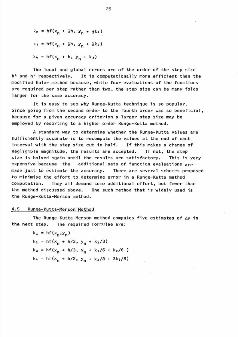
k2= hf(xn + Jh, Yn + Jkl)
k3
= hf(xn + Jh, Yn +
jk2)
k4= hf(xn + h, Yn +
k3)
The local and global errors are of the order of the step size
h' and h' respectively. It is computationally more efficient than the
modified Euler method because, while four evaluations of the functions
are required per step rather than two, the step size can be many folds
larger for the same accuracy.
It is easy to see why Runge-Kutta technique is so popular.
Since going from the second order to the fourth order was so beneficial,
because for a given accuracy criterion a larger step size may be
employed by resorting to a higher order Runge-Kutta method.
A standard way to determine whether the Runge-Kutta values are
sufficiently accurateis to
recomputethe
values atthe
end of eachinterval with the step size cut in half. If this makes a change of
negligible magnitude, the results are accepted. If not 'the step
size is halved again until the results are satisfactory. This is very
expensive because the additional sets of function evaluations are
made ust to estimate the accuracy. There are several schemes proposed
to minimise the effort to determine error in a Runge-Kutta method
computation. They all demandsome additional effort, but fewer than
the method discussed above. One such method that is widely used is
the Runge-Kutta-Merson method.
4.5 Runge-Kutta-Merson Method
The Runge-Kutta-Merson method computes five estimates of Ay in
the next step. The required formulae are:
ki = hf(x
nlyn)k2
= hf(xn+
h/3, Yn + ki/3)
k3
= hf(xn + h/3, yn+ ki/6 + k2/6
k4 = hf(xn+
h/2, yn+ ki/ 8+ 3k3/8)
8/6/2019 A. M. Y. Razak Thesis 1984
http://slidepdf.com/reader/full/a-m-y-razak-thesis-1984 44/181
30
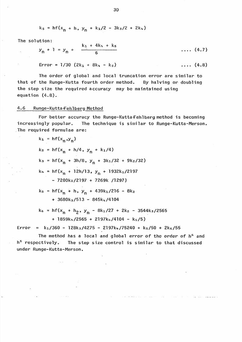
ks = hf(xn+h, Yn + ki/2 - 3k3/2 +
2k4)
The solution:
ki + 44 + k5Yn +I=yn+6 (4.7)
Error = 1/30 (2k, + 8k4 - k5)....
(4.8)
The order of global and local truncation error are similar to
that of the Runge-Kutta fourth order method. By halving or doubling
the step size the required accuracy may be maintained using
equation (4.8).
4.6 Runge-Kuttaf eh. berg Method
For better accuracy the Runge-Kuttaf eh berg method is becoming
increasingly popular. The technique is similar to Runge-Kutta-Merson.
-Therequired formulae are:
ki = hf (x
n3yn)k2
= hf(xn + h/4, yn+ ki/4)
k3 = hf(xn + 3h/8, yn+ 3k, /32 + 9k2/32)
k4 = hf(xn + 12h/13, yn+ 1932k, /2197
7200k2/2197 + 7269k /1297)
k5 = hf(x n 4- hl Yn + 439k1/216 - 8k2
3680k3/513 - 845k4/4104
k6 = hf(Xn +h 2' Yn - 8k1/27 + 2k2 - 3544k3/2565
1859k4/2565 + 2197k4/4104 - k5/5)
Error = ki/360 - 128k3/4275 2197k4/75240 + k5/50 + 2kG/55
The m thod has a local and global error of the order of h' and
h' respectively. The step size control is similar to that discussed
under Runge-Kutta-Merson.
8/6/2019 A. M. Y. Razak Thesis 1984
http://slidepdf.com/reader/full/a-m-y-razak-thesis-1984 45/181
31
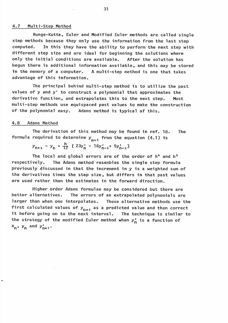
4.7 Multi-Step Method
Runge-Kutta, Euler and Modified Euler methods are called single
step methods because they only use the information from the last step
computed. In this they have the ability to perform the next step with
different step size and are ideal for beginning the solutions where
only the initial conditions are available. After the solution has
begun there is additional information available, and this may be storedin the memory of a computer. A multi-step method is one that takes
advantage of this information.
The principal behind multi-step method is to utilize the past
values of y and y' to construct a polynomial that approximates the
derivative function, and extrapolates this to the next step. Most
multi-step methods use equispaced past values to make the construction
of the polynomial easy. Adamsmethod is typical of this.
4.8 Adams Method
The derivation of this method may be found in ref. 18. The
formula required to determine yn+l
from the equation (4.1) is
hI+ TZ [ 23y 16y'_, + 5yn'n+l ý Yn
n-n -23
The local and global errors are of the order of h4 and h3
respectively. The Adamsmethod resembles the single step formula
previously discussed in that the increment in y is a weighted sum of
the derivatives times the step size, but differs in that past values
are used rather than the estimates in the forward direction.
Higher order Adams ormulae may be considered but there arebetter alternatives. The errors of an extrapolated polynomials are
larger than when one interpolates. These alternative methods use the
first calculated values of yn+1
as a predicted value and then correctit before going on to the next interval. The technique is similar to
the strategy of the modified Euler method when y' is a function ofn
x 3,y and y'nn n+1
8/6/2019 A. M. Y. Razak Thesis 1984
http://slidepdf.com/reader/full/a-m-y-razak-thesis-1984 46/181
32
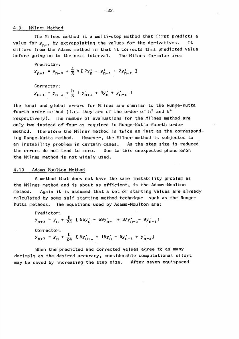
4.9 Milnes Method
The Milnes method is a multi-step method that first predicts a
value for yn+1
by extrapolating the values for the derivatives. it
differs from the Adamsmethod in that it corrects this predicted value
before going on to the next interval. The Milnes formulae are:
Predictor:
y 'I-Ah[
2yn' - yn'_1+
2yn_2+l
:- Yn-33
Corrector:
y+hyI+ 4y' +yn+l 'ý n-3.3 n+l n n'-l
The local and global errors for Milnes are similar to the Runge-Kutta
fourth order method (i. e. they are of the order of V and h4
respectively). The number of evaluations for the Milnes method are
only two instead of four as required in Runge-Kutta fourth order
method. Therefore the Milner method is twice as fast as the correspond-
ing Runge-Kutta method. However, the Milner method is subjected to
an instability problem in certain cases. As the step size is reduced
the errors do not tend to zero. Due to this unexpected phenomenon
the Milnes method is not widely used.
4.10 Adams-Moulton Method
A method that does not have the same instability problem as
the Milnes method and is about as efficient, is the Adams-Moulton
method. Again it is assumed that a set of starting values are already
calculated by some self starting method technique such as the Runge-
Kutta methods. The equations used by Adams-Moulton are:
Predictor:
y+h'- 59yn' + 37yn'n+' _2
9yn-3]n 55yn
Corrector:
yh[ 9y'+, + 19y' - 5y'_, +yn+l I- Yn + -f4- nnn n-23
When he predicted and corrected values agree to as many
decimals as the desired accuracy, considerable computational effort
may be saved by increasing the step size. After seven equispaced
8/6/2019 A. M. Y. Razak Thesis 1984
http://slidepdf.com/reader/full/a-m-y-razak-thesis-1984 47/181
33
values are available the step size may be conveniently doubled. When
the difference between the corrected and predicted value reaches or
exceeds the accuracy criterion the step size should be reduced. In
order to obtain the intermediate values when the step size is halvedthe following equation may be used where the local error is still of
the order of V.
IYn-J, =
TZ-8 [35yn+
140yn-i
- 70yn-2
+ 28yn-3 + 3y
n-4
Yn- 1-1
I-yn + 24yn-i-
+ 54yn-2
- 16yn-3+ 3y
n-42 64
It is clear that step size control using predictor corrector
methods are not as easy when comparedwith Runge-Kutta Merson or
Fehlberg methods. The disadvantages of these predictor corrector
methods are that they are not self-starting and the relative difficulty
in step size adjustment in order to satisfy a specified error criterion.
Nevertheless, the Adams-Moulton method is popular mainly because of its
better computational efficiency.
4.11 Hamming'sMethod
Another predictor corrector method that*has been widely accepted
is due to Hamming. The equations employed are:
y=y+ -ih[ 2yn' - yn'_, + 2yn_2
n+,,. n-3 3
Yn+3.in
= Yi+,, - 112 1Yn, - Yn,c121
p
=11 9y + 3h(ynn'+i,m
+ 2ynon
Ynn+l,,8n-
Yn-2'-1)3
9Yn+l ý Yn+l,
c+121
(yn+l,
p-Yn+i,
ýc
The predictor equation is the Milner predictor. Before
correcting the estimated value, Yn+1,
it is modified using the differ-
ence between the predicted and corrected values of the previous
8/6/2019 A. M. Y. Razak Thesis 1984
http://slidepdf.com/reader/full/a-m-y-razak-thesis-1984 48/181
34
interval, yn+1,
m.
Although two additional equations appear in each
step compared wth the other predictor-corrector methods discussed,
only two evaluations of the derivative functions are needed as before.
Therefore the Hemming'smethod is as computationally efficient as the
Milnes and Adams-Moulton methods.
The special merits of the Hammingsmethod are good stability
combined with good accuracy. Like the Adams-Moulton and the Milnes,
the method has a local and global error of the order of h5 and h4
r.espectively.
4.12 Gears Method
Gears (ref. 19) has proposed a predictor-corrector method that
has a local error of the order of h' using only three previous steps
rather than four as employed by Adams-Moulton and Milnes. It obtains
its high accuracy by recorrecting values for the function and
derivatives. The formulae employed are:
Yn+l, pý-
18Yn+
9yn-1, c+
loyn-l, c2+
9hyn'
18hyj_1 + 3hyj-2
hy,1 -57yn+
24yn-i,
c+
33yn-2, C
2.1
24hyn' + 57hyn'_, + 10hyn_2
F= hyn'+l,
p-
hf (xn+i,
Yn+l,p)
Yn+l `ý y-95
Fn+l,
p288
yn,
cl n
Yn-1,C2
yn-i-scl
_11
FT4-4U
hyn'+l ý hyn'+i,
p-F
8/6/2019 A. M. Y. Razak Thesis 1984
http://slidepdf.com/reader/full/a-m-y-razak-thesis-1984 49/181
8/6/2019 A. M. Y. Razak Thesis 1984
http://slidepdf.com/reader/full/a-m-y-razak-thesis-1984 50/181
- 36
CHAPTER5
5.0 EXPERIMENTALALIDATIONOFTHE-MATHEMATICALODEL
An experimental program was undertaken to validate the
mathematical model developed in Chapter 2.0. The experiment was
conducted using a turbo-charger.
5.1 Description of Test Rig and Instrumentation
In order to obtain useful results a very simple system was
chosen for the experimental study. The test rig is shown
in fig. 5.1.
The compressor was a small (100mmmpeller diameter), single
stage, centrifugal compressor. The compressor speed selected for the
test was 90,000 rpm. The characteristic of the compressor at thechosen speed is shown in fig. 5.2.
The duct work upstream of the compressor consisted of a
straight pipe and an inlet bell mouth. The downstream ducting had two
right angle bends and a branch to which a fast acting blow-off valve
was mounted. (The valve stroke times for the opening and closing ofthe blow-off valve were 0.25 seconds. and 0.5 seconds respectively. )
The blow-off valve was a repeatable poppet actuator type, and fasttransients were introducted into the system by the operation of this
valve. The compressor delivery air exhausted through a throttle
valve, and the compressor steady state operating point on its character-istic was determined by the actuation of this throttle valve.
High performance pressure transducers were mounted at the
system inlet, impeller inlet, compressor outlet and blow-off valve
stations respectively. The type of transducers used is given inAppendix A. These transducers were calibrated and the expression
for pressure as a function of voltage is also given in Appendix A.
Due to the relative small changes in pressure ratios during the
transients considered and the slowness of the temperature changes the
8/6/2019 A. M. Y. Razak Thesis 1984
http://slidepdf.com/reader/full/a-m-y-razak-thesis-1984 51/181
37
effect of temperature on the pressure readings were neglected. All
the data from the transducers were stored on magnetic tape using the
system shown in fig. 5.3.
The duct work upstream of the turbine section was a straight
pipe via a combustion chamber connecting to the high pressure air
supply. The exhaust from the turbine was discharged via a straight
vertical pipe to the ambient. The combustion chamber becomes
operational if insufficient energy is available in the high pressure
air (cold) driving the compressor at the required speed and pressure
ratio (preheating using the combustion chamber was required for operating
conditions above 60,000 RPM).
5.2 Compressor Test
A series of validation tests were conducted. Firstly, by
adjusting the flow through the throttle valve (fig. 5.1) a steady state
compressor operating point on the compressor was chosen, point A in
fig. 5.2. A this operating point the flow through the compressor wasmeasured to be 0.54 kg s-1 at a-pressure ratio of 3.3. The blow off
valve was set to the closed position.
5.3 Compressor Transients between Stable Points
By the actuation of the blow-off valve a fast transient was
introduced into the system. The repeated opening and closing of the
blow-off valve transients between the corresponding two stable points
were obtained. Sufficient time was given between the opening and
closing of the valve so that the post transient steady state operating
point could be obtained. During the transient the compressor speed
remained nominally constant. The stable points due to the opened and
closed position of the blow-off valve are shown by point A and B
respectively in fig. 5.2.
5.4 Surge'Tests
The blow-off valve was returned to the opened position, and by
adjusting the flow through the throttle valve in fig. 1 the compressor
was made to operate at point A (fig.. 5.2) on the characteristic. The
8/6/2019 A. M. Y. Razak Thesis 1984
http://slidepdf.com/reader/full/a-m-y-razak-thesis-1984 52/181
38
transient due to the closing of the blow-off valve was sufficient to
take the compressor into surge. The compressor remained under surge
conditions for only approximately 15 seconds so that no damagewas
done to the test rig. This surge test was repeated twice.
5.5 Data Analysis
The analogue signals from the pressure transducers during the
transient were stored on magnetic tape. A separate channel on the
tape recorder was used for each transducer. The tape recorder also
stored a trigger pulse which was produced whenever a transient was
initiated.
The stored signal was passed through an oscilloscope so that
the beginning of a transient could be defined. From the oscilloscope
the signal was sent to a DATA-LABDL905 transient recorder. The
digitised output from the transient recorder was stored on floppy disk
via a PET2001 micro computer (see fig. 5.3). The program package used
in the micro computer known as "DATA" is described in ref. (20).
Having determined the beginning of the transient, the magnetic
tape was played back again, however, on this occasion the transient
recorder was armed and the computer program executed. In this con-
dition the transient recorder waits for the trigger pulse. When he
transient recorder received the trigger pulse and starts digitising
(the analogue signal from the tape recorder) the micro computer waits
until all data has been accepted by the transient recorder. The micro
computer then goes into the final stages of transfering the digitised
data from the transient recorder into its memory and then on to the
floppy disk. This was repeated for each data channel on the recorder.
The compressor transients considered were very fast. The
section of the magnetic tape which represented ten seconds after the
transient was initiated was taken for digitisation. To achieve this
a sweep time of ten seconds was set on the DATA-LABransient recorder.
In this time period the analogue signal was digitised into 1024 parts
which range from 0 to 255 in value. The nature of the signal being digitised
may give rise to the situation where this range is exceeded, hence intro-
ducing an overflow condition in the micro computer. To overcome this,
an off-set and a scaling of the voltage was introduced to provide the
8/6/2019 A. M. Y. Razak Thesis 1984
http://slidepdf.com/reader/full/a-m-y-razak-thesis-1984 53/181
39
correct level of signal. An offset of 124 and a scaling of the voltage
of 2 volts was sufficient to ensure that the signal was within the given
range. A flow chart explaining how the transient recorder and the
micro computer interact is shown in fig. 5.4.
The next task was to convert the digitised data into pressure
readings. A computer program was developed using the micro computer
incorporating the characteristics of the pressure transducers. The
program was structured into different subroutines where each sub-
routine determined the pressures from the digitised data that origin-
ated from a particular transducer. Such a structure was chosen so
that further transducers may be incorporated into the program with
ease. A flow chart describing this is shown in fig. 5.5.
The output from this program may be in a printed format of
pressure readings and time, or a simple graphical output. To obtain
the graphical output the TAB function was used. The variable
incorporated in the TAB function was the digitised number rather than
the pressure value. The reason for this being that the TAB function
is only accurate to the nearest integer and therefore the full
transient may be captured using the digitised number. The scale of
the graph was, however, calibrated in pressure units (pa) using the
characteristics of the transducer. The graphical output enabled one
to select an interesting transient to simulate with relative ease.
5.6 Simulationof Compressor Transients
The mathematical model described in Chapter 2 was implemented
in a Fortran IV program using a PDP11/34 machine. The system shown
in Fig. 5.1 was discretised into elements using the frequency parameter
and approximately equal volume concept discussed in Chapter 3. The
element geometry was selected such that the system had a frequency
response of 200 Hz, although the frequency response expected during
the transient need not exceed about 150 Hz. The system is schemat-
ically represented in Fig 5.6 and the geometry of the elements withinthe system is given in appendix B.
5.7 Settinq Up of Data for Simulation
The simulation program is in two parts. The first, whose name
8/6/2019 A. M. Y. Razak Thesis 1984
http://slidepdf.com/reader/full/a-m-y-razak-thesis-1984 54/181
40
is "SETUP", sets up the data files required for the second program
"TRANS",where the simulation is performed. The program SETUPs
divided into five sections. The first part reads the gas properties
such as the gas constant R, gamma , specific heat Cp, system entry
pressure, temperature and various times (eg. valve stroke time, valve
movement ime etc. ). The next part reads the number of elements in
the system, number of compressor stages and compressor speed.
The third part of the program, SETUP,enables the simulation
program TRANSo distinguish one type of element from another, by
associating a number to each type of element that exists in the system.
Appendix (B) shows the-different types of elements that are involved
in representing the system. The meaning of these elements are as
follows.
a) Duct-with-loss (TYPE= -2)
This element is used to represent pipe work which only
introduces a pressure loss. The pressure loss is determined using
pipe resistance coefficients and the technique used to determine the
pressure loss is given in*Chapter 3.
b) Blow-off-valve (TYPE = -3)
This element is used to introduce a transient into the system.
The dynamic response of this element was neglected as it was considered
to be sufficiently small. The relationship for the valve movement
are givenin Chapter 3
andthis information
maybe
obtainedfrom the
valve manufacturer.
c) Compressor (TYPE= 1)
This is the only element that inputs work into the system.
The pressure rise across this element is determined from its pressure
rise characteristic. During the development of the program it was
decided that the compressor characteristic should be of the form of
polytropic head against volume flow rate. The reason being that
most industrial compressors have characteristics expressed in this
form.
8/6/2019 A. M. Y. Razak Thesis 1984
http://slidepdf.com/reader/full/a-m-y-razak-thesis-1984 55/181
41
These were the only type of elements needed for the simulation
of the test rig. However, other elements which represent recycle
valves, non-return valves, branch, bends etc. are also available(Appendix C).
The next selection of the program reads the geometry of each
element and loss constants as the pressure drop in the element were
to be defined by experimental values (ie. element type -4 duct with
experimental loss DWELn Appendix C).
The compressor stage characteristics are input to the program
followed by the compressor speed time history. This speed time history
accounts for any variation in compressor speed during the transient.
However, the compressor speed remained nominally constant during this
test but any such variation in speed may be included without analysing
the dynamic response of the driver (in this case, the turbine). The
data is stored on floppy disks by generating two data files. The first
stores the system variable and the other stores the speed history only.
This choice was made so that if a few variables need changing in the
system this could be achieved by editing the system variable data file
using the computer command odes. It is also possible to make the
necessary changes to the file by executing the data program SETUP. A
flow chart describing SETUPs given in Fig. 5.7. A typical data file
is given in Table 5.1with a guide to the meanings of the variables in
that file, in Appendix D).
5.8 The Simulation Program TRANS
The simulation program consists of a main routine which calls
the necessary subroutines defining the type of elements that exist in
the data files generated by SETUP. Further to this the integrating
section has been included as a separate subroutine. Such a structure
enables the inclusion of other integrating algorithms and new types of
elements with relative ease.
A flow chart describing program TRANS fig. 5.8) shows that it is
split up at point 'A' into two sections. The first section reads in
all the data, performs a curve fit upon any element characteristic
using a natural cube spline fit, and sets up the initial valves of the
8/6/2019 A. M. Y. Razak Thesis 1984
http://slidepdf.com/reader/full/a-m-y-razak-thesis-1984 56/181
42
element variable to give steady state ýunning conditions. These tasks
are performed once per program run.
The second section of the program contains the call for the
integrating routine (subroutine RKM,see Appendix E) where the bulk of
the calculations are performed during a program run. Most of the
calculations necessary to simulate the transients occur with subroutines
RKM,SUB01and DYBDX.
The program path is determined by two 'If' statements. The
first of these enables the change of certain variables (eg. pressure,
temperature, mass flow and gas properties of any element within the
system) using subroutine SUB06(see appendix E), at a simulated time
specified by the initial input data variable XTIM (see typical data file
Table 5.1). Since XTIMmay be reset within subroutine SUB06 t is
possible to simulate a sequence of transient inducing events.
The second 'If' statement determines whether an output should
occur. In order to reduce computer output. and hence computer run
times an output occurs if the fixed output interval (OUTDEL,defined in
the data file, Appendix D) is reached, or if the ratio of the compressor
entry mass to the time changes sign. This enables all the oscillatory
response during a transient to be captured.
5.9 Program Performance
The main problem encountered is one of program-run times and
hard copy times, where a single simulation may take several hours.
Fortunately, this problem is to a large extent dependent on the type of
computer used and its peripheral equipment. The reduction of computer
time is in someways a simple matter of employing a more powerful
computer. To test this theory the TRANS rogram was executed using a
VAX 11/780 machine. The CPUtime was reduced by some85%.
The problem of run time is also a function of the number of
elements used to define the system. Generally the computer runtime
increases proportionally with the number of elements within a system.Only five elements were required for the validating simulation, however
if a real process plant were to be considered, and indeed the case of
the gas transmission station considered in Chapter 6, the number of
elements may run into hundreds. Under these conditions the impressive
8/6/2019 A. M. Y. Razak Thesis 1984
http://slidepdf.com/reader/full/a-m-y-razak-thesis-1984 57/181
43
reduction in computer run times achieved using the VAX 11/780 machine
still represents a run time of over an hour.
Another line of attack on computer run times is to use a faster
integrating algorithm. The method used in program TRANSs the Runge-
Kutta-Merson. The main reason for the use of this method of integrat-
ion is the ease of integrating step size control to keep the error
within some pre-set limit. However,. Runge-Kutta-Merson is by no means
the fastest method numerical integration.. Another desirable feature
of Runge-Kutta -Merson is that the method is self-starting unlike
predictor-corrector methods such as Adam-Moulton, Hammingand Gears.
This disadvantage of starting predictor-corrector methods is notinherent in this case, the reason being that the system considered for
simulation is initialised to give steady state response. Therefore,
the previous values for the rates of change may be conveniently put to
zero and hence the previous solutions are also known. Generally, these
predictor; corrector methods are some60% aster than Runge-Kutta-Merson
but the change in step size , so that the integration error will be
below a pre-determined limit,is
not that easy. The reasonbeing
thatthe previous values needed for most predictor-corrector methods must be
of equal step. Therefore, one must interpolate and extrapolate to
ensure good accuracy. The general rule is that if stable solutions
are found then the integrating error is relatively small, hence making
such predictor-corrector methods attractive in achieving small computer
run times. Another attractive property of prediction-correction
methods such as Hammingand Gears, are that they are well suited for
so-called stiff equations, discussed in Chapter 4.0.
An altogether different approach in reducing large computer run
times is the application of the concept of parallel or array processing.
Basically, this approach enables the computer to evaluate a sequence
of events by one instruction. Therefore if 'n' elements were involved
in defining a system, array processing will be able to complete the
task in approximately 1/nth the time required by conventional computers
that operate on a sequential basis. However, this technique is only
useful when many hundreds of elements are involved in the system.
Ref. 21 and 22 give details on array processing.
8/6/2019 A. M. Y. Razak Thesis 1984
http://slidepdf.com/reader/full/a-m-y-razak-thesis-1984 58/181
44
5.10 The Simulation of Measured Transients
The following transients were simulated to provide a comparison
between the experimental data obtained and the model prediction.
(i) Point to Point Simulation
a) The model was set up so that the compressor operated at point 'A'
on the compressor characteristic (fig. 5.2). After 0.2 seconds of
steady state running a transient was introduced by opening the blow off
valve. The post transient steady state compressor operating point is
also shown in fig. 5.2 by point W.b) Next the operating of the compressor on its characteristic was set
at point W, (fig. 5.2) with the blow off valve in the opened position.
Again after 0.2 seconds of steady state running a transient was
initiated by the closure of the blow off valve element, and therefore
reproducing the two steady state compressor operating points 'A' and
'B' on the compressor characteristic.
(ii) Surge Simulation
Compressor surge, the periodical reversal of flow within the
compressor, is by far, the most dangerous aspect of compressor operation.
Therefore its prediction is of vital importance within the simulating model.
For successful simulation of compressor surge the unstable part
of the compressor characteristic is required. The reasons being that
the force terms, Fnet, in equation (3.5) in chapter (3) are determined bythe interpolation of the compressor characteristic. However, the un-
stable part of the characteristic is exceedingly difficult to obtain by
experimental means. By understanding how surge cycles are formed the
shape of the unstable part of the compressor characteristic may be
estimated.
Fig. 5.9 shows a typical form of a compressor characteristic
operating at constant speed. Using this diagram the behaviour of adynamic compressor delivering gas through a pipe downstream operating
under surge conditions can be explained. The unstable region wherethe characteri sti c has a posi ti ve s1ope 1i es between poi nts A and C.
As the operating point moves from D to A, a reduction in gas flow is
8/6/2019 A. M. Y. Razak Thesis 1984
http://slidepdf.com/reader/full/a-m-y-razak-thesis-1984 59/181
8/6/2019 A. M. Y. Razak Thesis 1984
http://slidepdf.com/reader/full/a-m-y-razak-thesis-1984 60/181
46
It is interesting to note that a similar conclusion was reached in
ref. 7
The simulated and experimental results for the surge cyclesare shown n Fig. 5.13atthe compressor delivery and blow-off valve
station. The discrepancy in frequency between the experimental and
simulated values are small, and the periodic time of the oscillation
for both cases are equal to the time taken for a pressure wave to
propagate the length of the system and back. The slight difference
in time to surge between the simulated and experimental results can
again be attributed to the inaccuracy in the blow-off valve relation.
Fig 5.14 showsthe resultant surge cycle on the compressor characteristic.
A series of further surge cycle simulation was repeated,
however the compressor volume was changed by ± 20% in steps of 5%.
These simulated results when compared with the experimental tests
showed small errors up to ± 10%change in compressor volume. This
feature is very valuable as it is not always possible to obtain the
compressor geometry very accurately, due to the tortuous path the gas
follows within the compressor. Therefore, if an accuracy in
compressor geometry of ± 10% s obtained it could be concluded that
the simulation is still largely-valid.
5.12 Conclusions
The simulated results compare favourably with those of the
experimental tests. The small discrepancies are mainly attributed to
the inaccuracies in the representation of the poppet valve action.
The travel of the poppet valve was assumedto be linear with time. In
reality the valve action is likely to be of the form
displacement a(time)n
where n>1
This valve information was exceedingly difficult to obtain and
a linear response of the valve was assumed. Due to small valve stroke
times of the poppet valve the error introduced due to this linear
8/6/2019 A. M. Y. Razak Thesis 1984
http://slidepdf.com/reader/full/a-m-y-razak-thesis-1984 61/181
47
assumption is small.
Surge tests gave good results. The frequency response of the
system between simulated and experimental results were good.
With satisfactory validation results, the model was then applied
to a British Gas transmission station. - This'pliknt was
selected because it had operational problems associated with plant
dynamics. The simulation of the gas transmission station was discussed
in chapter 6.0.
8/6/2019 A. M. Y. Razak Thesis 1984
http://slidepdf.com/reader/full/a-m-y-razak-thesis-1984 62/181
48
CHAPTER
6.0 APPLICATIONOF THEMODEL O SIMULATE HEDYNAMIC ESPONSEF
THEGASTRANSMISSIONTATION
The operation of the transmission station suffered compressor
stability problems and it was a problem that manifested itself when new
compressor wheels and non-return valves were installed. The model was
used to investigate the problem and suggest solution in order that the
system may operate satisfactory. The first part of this chapter discusses
the extention and validation of the program so that the gas transmission
may be considered.
6.1 Further Development of Program
The program developed to this point was only capable of simulating
the dynamic response of compressor systems used in series, (i. e. flow
enters at station 1 and leaves from the last station). Many practical
examples, however, use compressor systems which are connected in parallel,
(with parallel flow paths) and therefore the computer model had to be ableto simulate such systems. To achieve this the program was modified such
that any number of "series" systems may be connected together to simulate
parallel paths. This was achieved using a patching routine.
Consider the compressor system shown in Fig. 6.1 where three
compressors may operate in parallel and each compressor discharges to
a commonoutlet. Firstly, by applying the frequency and equal volume
concepts, discussed in Chapter 3, the whole system is divided into
elements whose geometry is defined by the frequency response of the
system. Secondly the element types are assigned to each element (e. g.
duct with loss, bend, compressor, tee-section, etc. ). Since the
procedure for connecting the series systems are only required at a branch
junction (or tee section), the patching routine is invoked only when this
element is located. To achieve this the patching routine is included
inthe subroutines
describing thepressure
loss in the tee-piece.
6.2 Patching Procedure
The system shown in Fig. 6.1 is divided into three series paths
AB, CEDand EF, where AB is considered the main system and CED, EF
8/6/2019 A. M. Y. Razak Thesis 1984
http://slidepdf.com/reader/full/a-m-y-razak-thesis-1984 63/181
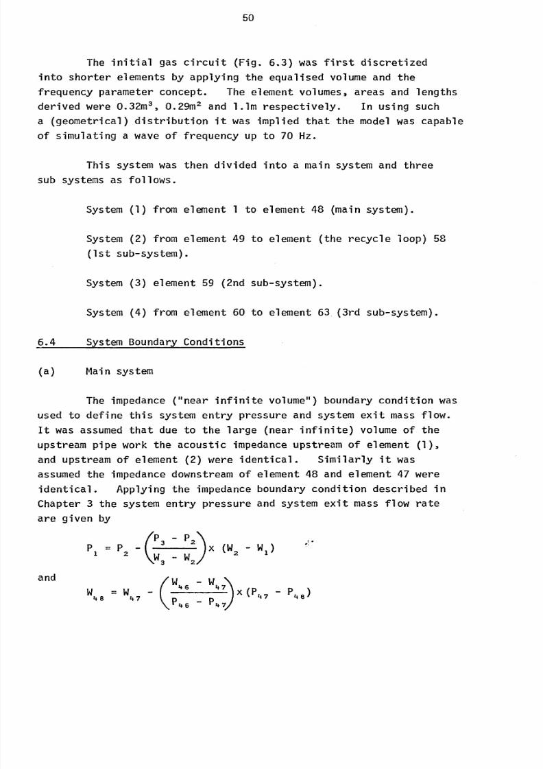
8/6/2019 A. M. Y. Razak Thesis 1984
http://slidepdf.com/reader/full/a-m-y-razak-thesis-1984 64/181
50
The initial gas circuit (Fig. 6.3) was first discretized
into shorter elements by applying the equalised volume and the
frequency parameter concept. The element volumes, areas and lengths
derived were 0.32M3,0.29M2 and 1.1m respectively. In using such
a (geometrical) distribution it was implied that the model was capable
of simulating a wave of frequency up to 70 Hz.
This system was then divided into a main system and three
sub systems as follows.
System (1) from element 1 to element 48 (main system).
System (2) from element 49 to element (the recycle loop) 58
(1st sub-system).
System (3) element 59 (2nd sub-system).
System (4) from element 60 to element 63, (3rd sub-system).
6.4 System Boundary Conditions
(a) Main system
The impedance ("near infinite volume") boundary condition was
used to define this system entry pressure and system exit mass flow.
It was assumed that due to the large (near infinite) volume of the
upstream pipe work the acoustic impedance upstream of element (1),
and upstream of element (2) were identical. Similarly it was
assumed the impedance downstream of element 48 and element 47 were
identical. Applying the impedance boundary condition described in
Chapter 3 the system entry pressure and system exit mass flow rate
are given by
P, =p
ýP3
P2x (W
2-WI)
w3w2)
and
WW
(W46-
W41
X (P47-
P48)
48 47 P46-
P4
)
7
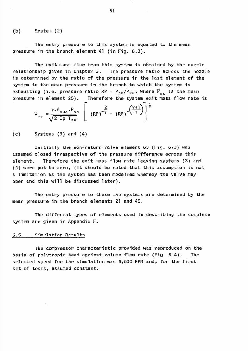
8/6/2019 A. M. Y. Razak Thesis 1984
http://slidepdf.com/reader/full/a-m-y-razak-thesis-1984 65/181
51
(b) System (2)
The entry pressure to this system is equated to the mean
press ure in the branch element 41 (in Fig. 6.3).
The exit mass flow from this system is obtained by the nozzle
relationship given in Chapter 3. The pressure ratio across the nozzle
is determined by the ratio of the pressure in the last element of the
system to the mean pressure in the branch to which the system is
exhausting (i. e. pressure ratio RP = P,, /P,,,, where F2. is the mean
pressure in element 25). Therefore the system exit mass flow rate is
y. Anoz*
p2(1+1
w58 2 Cp T58
(RP)-y - (RP)-V Y
(C) Systems (3) and (4)
i
Initially the non-return valve element 63 (Fig. 6.3) was
assumed closed irrespective of the pressure difference across this
element. Therefore the exit mass flow rate leaving systems (3) and
(4) were put to zero, (it should be noted that this assumption is not
a limitation as the system has been modelled whereby the valve may
open and this will be discussed later).
The entry pressure to these two systems are determined by themean pressure in the branch elements 21 and 45.
The different types of elements used in describing the complete
system are given in Appendix F.
6.5 Simulation Results
The compressor characteristic provided was reproduced on the
basis of polytropic head against. volume flow rate (Fig. 6.4). The
selected speed for the simulation was 6,500 RPMand, for the first
set of tests, assumed constant.
8/6/2019 A. M. Y. Razak Thesis 1984
http://slidepdf.com/reader/full/a-m-y-razak-thesis-1984 66/181
52
A series of validation tests were conducted as follows.
6.6 Action of Recycle Valve
A transient was introduced by opening the recycle valve (element
55 in Fig. 6.3) with the compressor operating at point (1) on the
compressor characteristic (see Fig. 6.4). The steady state operating
point with the recycle valve open is indicated by point (2) on the
compressor characteristic (Fig. 6.4). To reduce computing time the
action of the recycle valve was considered infinitely fast. The
stagnation pressure variation atthe
compressorinlet
and outletstation (Fig. 6.5a) prompt the following comments
(1) The compressor outlet pressure fall (due to the opening of the
recycle valve) was not very large because of the relatively
flat compressor characteristic.
(2) During the transient the compressor inlet pressure decreased
a little. This is apparently due to increased losses in the
intake system associated with increase in mass flow through
that system. Operation at both points (1) and (2) on the
compressor characteristic (Fig. 6.3) were quite stable.
6.7 Effect on Non-Return Valve due to the action of Recycle Valve
It was suspected that during the actuation of the recyclevalve the non-return valve could open or flap. To determine whether
the pressure difference across the non-return valve (element 63 in
Fig. 6.3) could cause this valve to becomeactive the pressure time
history for this element was iývestigated (Fig. 6.5b). It can be
seen that the pressure difference across this valve is always large
ensuring that it remains closed during the transient.
6.8 Transient Responsedue to Perturbation
The operating point on the compressor characteristic was moved
to point (3) (see Fig. 6.4) and the, recycle valve to the closed position.
The system was then perturbed by altering the pressure instantaneously
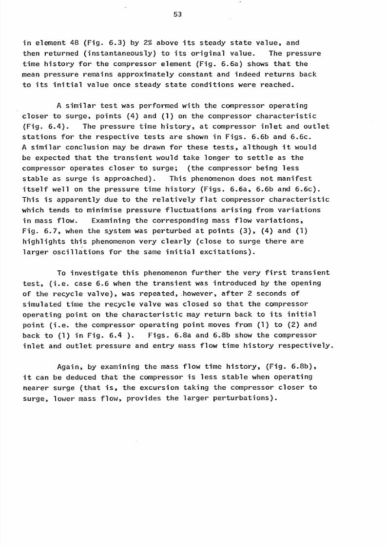
8/6/2019 A. M. Y. Razak Thesis 1984
http://slidepdf.com/reader/full/a-m-y-razak-thesis-1984 67/181
53
in element 48 (Fig. 6.3) by 2%above its steady state value, and
then returned (instantaneously) to its original value. The pressure
time history for the compressor element (Fig. 6.6a) shows that the
mean pressure remains approximately constant and indeed returns backto its initial value once steady state conditions were reached.
A similar test was performed with the compressor operating
closer to surge, points (4) and (1) on the compressor characteristic
(Fig. 6.4). The pressure time history, at compressor inlet and outlet
stations for the respective tests are shown in Figs. 6.6b and 6.6c.
Asimilar conclusion may
be drawn for these tests,although
itwould
be expected that the transient would take longer to settle as the
compressor operates closer to surge; (the compressor being less
stable as surge is approached). This phenomenondoes not manifest
itself well on the pressure time history (Figs. 6.6a, 6.6b and 6.6c).
This is apparently due to the relatively flat compressor characteristic
which tends to minimise pressure fluctuations arising from variations
in mass flow. Examining the corresponding mass flow variations,
Fig. 6.7, when the system was perturbed at points (3), (4) and (1)
highlights this phenomenonvery clearly (close to surge there are
larger oscillations for the same initial excitations).
To investigate this phenomenon urther the very first transient
test, (i. e. case 6.6 when the transient was introduced by the opening
of the recycle valve), was repeated,. however, after 2 seconds of
simulated time the recycle valve was closed so that the compressoroperating point on the characteristic may return back to its initial
point (i. e. the compressor operating point moves from (1) to (2) and
back to (1) in Fig. 6.4 ). Figs. 6.8a and 6.8b show the compressor
inlet and outlet pressure and entry mass flow time history respectively.
Again, by examining the mass flow time history, (Fig. 6.8b),
it can be deduced that the compressor is less stable when operating
nearer surge (that is, the excursion taking the compressor closer to
surge, lower mass flow, provides the larger perturbations).
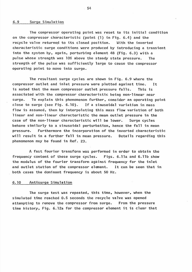
8/6/2019 A. M. Y. Razak Thesis 1984
http://slidepdf.com/reader/full/a-m-y-razak-thesis-1984 68/181
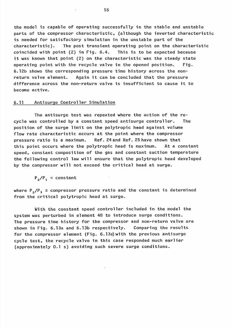
8/6/2019 A. M. Y. Razak Thesis 1984
http://slidepdf.com/reader/full/a-m-y-razak-thesis-1984 69/181
55
the model is capable of operating successfully in the stable and unstable
parts of the compressor characteristic, (although the inverted characteristic
is needed for satisfactory simulation in the unstable part of the
characteristic). The post transient operating point on the characteristic
coincided with point (2) in Fig. 6.4. This is to be expected because
it was known that point (2) on the characteristic was the steady state
operating point with the recycle valve in the opened position. Fig.
6.12b shows the corresponding pressure time history across the non-
return valve element. Again it can be concluded that the pressure
difference across the non-return valve is insufficient to cause it to
becomeactive.
6.11 Antisurge Controller Simulation
The antisurge test was repeated where the action of the re-
cycle was controlled by a constant speed antisurge controller. The
position of the surge limit on the polytropic head against volume
flow rate characteristic occurs at the point where the compressor
pressure ratio is a maximum. Ref. 24and Ref. 25 have shown that
this point occurs where the polytropic head is maximum. At a constant
speed, constant composition of the gas and constant suction temperature
the following control law will ensure that the polytropic head developed
by the compressor will not exceed the critical head at surge.
p2 /Pl < constant
where P21PI -=compressor pressure ratio and the constant is determined
from the critical polytropic head at surge.
With the constant speed controller included in the model the
system was perturbed in element 48 to introduce surge conditions.
The pressure time history for the compressor and non-return valve are
shown in Fig. 6.13a and 6.13b respectively. Comparing the resultsfor the compressor element (Fig. 6.13a)with the previous antisurge
cycle test, the recycle valve in this case responded much earlier
(approximately 0.1 s) avoiding such severe surge conditions.
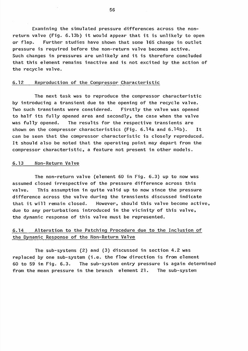
8/6/2019 A. M. Y. Razak Thesis 1984
http://slidepdf.com/reader/full/a-m-y-razak-thesis-1984 70/181
56
Examining the simulated pressure differences across the non-
return valve (Fig. 6.13b) it would appear that it is unlikely to open
or flap. Further studies have shown that some 16%change in outlet
pressure is required before the non-return valve becomesactive.
Such changes in pressures are unlikely and it is therefore concluded
that this element remains inactive and is not excited by the action of
the recycle valve.
6.12 Reproduction of the Compressor Characteristic
The next task was to reproduce the compressor characteristicby introducing a transient due to the opening of the recycle valve.
Two such transients were considered. Firstly the valve was opened
to half its fully opened area and secondly, the case when the valve
was fully opened. The results for the respective transients are
shown on the compressor characteristics (Fig. 6.14a and 6.14b). It
can be seen that the compressor characteristic is closely reproduced.
It should also be noted that the operating point may depart from the
compressor characteristic, a feature not present in other models.
6.13 Non-Return Valve
The non-return valve (element 60 in Fig. 6.3) up to now was
assumed closed irrespective of the pressure difference across this
valve. This assumption in quite valid up to now since the pressure
difference across the valve during the transients discussed indicate
that it will remain closed. However, should this valve becomeactive,
due to any perturbations introduced in the vicinity of this valve,
the dynamic response of this valve must be represented.
6.14 Alteration to the Patching Procedure due to the Inclusion of
the Dynamic Response of the Non-Return Valve
The sub-systems (2) and (3) discussed in section 4.2 was
replaced by one sub-system (i. e. the flow direction is from element
60 to 59 in Fig. 6.3. The sub-system entry pressure is again determined
from the mean pressure in the branch element 21. The sub-system
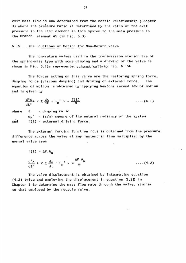
8/6/2019 A. M. Y. Razak Thesis 1984
http://slidepdf.com/reader/full/a-m-y-razak-thesis-1984 71/181
57
exit mass flow is now determined from the nozzle relationship (Chapter
3) where the preisure ratio is determined by the ratio of the exit
pressure in the last element in this system to the mean pressure in
the branch element 45 (in Fig. 6.3).
6.15 The Equations of Motion for Non-Return Valve
The non-return valves used in the transmission station are of
the spring-mass type with somedamping and a drawing of the valve is
shown in Fig. 6.15a represented schematically by Fig. 6.15b.
The forces acting on this valve are the restoring spring force,
damping force (viscous damping) and driving or external force. The
equation of motion is obtained by applying Newtons second law of motion
and is*given by
d2x+2,
dx+wIxf
(t)
dt'HE nm
where = damping ratio
wn' = (s/m) square of the natural radiancy of the system
and f(t) = external driving force.
The external forcing function f(t) is obtained from the pressure
difference across the valve at any instant in time multiplied by the
normal valve area
f (t) = AP.AN
d2-x
+2CýX
+2X
4P.AN
dt' dt nm(4.2)
The valve displacement is obtained by integrating equation
(4.2) twice and employing the displacement in equation 0.21) in
Chapter 3 to determine the mass flow rate through the valve, similar
to that employed by the recycle valve.

8/6/2019 A. M. Y. Razak Thesis 1984
http://slidepdf.com/reader/full/a-m-y-razak-thesis-1984 72/181
58
6.16 Validation of Non-Return Valve
A transient was introduced into the system by perturbing the
high pressure side of the non-return valve (element 63 in Fig. 6.3),such that the pressure in the high pressure side was reduced instantly
to 400 kpa after 0.02 seconds of steady state running with constant
compressor speed operation. This perturbation was sufficient to open
the non-return valve and the resultant pressure time history across
the non-return valve is shown in Fig. 6.16. Since this pressure
restraint on the high pressure side of the valve is only instantaneous
and the compressor continuing to deliver gas at a higher pressure
the tendency is to close the non-return valve. When he pressure
difference across the non-return valve is sufficient to keep it closed
the system returns to the initial conditions, and this can be seen in
Fig. 6.17, where the pressure time histIory for the non-return valve is
plotted on a smaller time scale.
The corresponding valve movement and the mass flow rate through
the non-return valve is shown in Figs. 6.18a and 6.18b respectively.
It is interesting to note that the mass flow rate does not reach a
maximumwhen the valve is fully opened. The natural frequency of
the spring-mass system in the non-return valve is some 3 Hz. The.
perturbing or forcing function frequency is some 50 Hz. This condition
gives rise to a phase shift between the valve movementand the forcing
function. Therefore the pressure difference across the valve will be
a minimum when the valve movement is a maximum. Since the massflow
through the valve is a product of somefunction of the pressure difference
across the valve and the valve movement, (equations 3.21 and 3.22 in
Chapter 3, this unexpected phenomenonoccurs. This phase shift is
not quite 7T radians and is due to the initial transient response
of the valve movement.
6.17 Variable Speed Simulation
The compressor characteristic at different speeds are of similar shape,
Fig. 6.4. This feature enables the lower speed characteristics to
be obtained by assuming that the polytropic head and the volume flow
8/6/2019 A. M. Y. Razak Thesis 1984
http://slidepdf.com/reader/full/a-m-y-razak-thesis-1984 73/181
59
rate vary according to the square of the compressor speed and linear to
the compressor speed respectively. This assumption is valid for
compressors that operate at low pressure ratios, typically up to 2.0.
The pressure of the compressor never exceeds this value and therefore
above assumption is valid for the compressor employed in the trans-
mission station.
The speed transients were introduced by reducing the compressor
speed linearly. The deceleration was taken as 500 rpm per second
(as opposed to a more usual rate of deceleration of 5 rpm per second)
in order to keep computing time to a reasonable level.
The compressor operating point was set at point (4) on the
characteristic, Fig. 6.4, and the speed transient was introduced after
0.02 seconds of steady state running. Fig. 6.19a and Fig. 6.19b
show the variation of inlet, outlet pressure and entry mass flow rate
for the compressor element respectively. The operating point on the
compressor characteristic during this transient is also shown in
Fig. 6.20.
The transient running line on the compressor characteristic is
almost horizontal, and is imposed largely by a near infinite capacity
of the downstream duct work.
Another speed transient test was also simulated, however in
this case the impedance boundary condition in element 48 (Fig. 6.3)
was replaced by a nozzle condition. The system. discharges through
this nozzle to a fixed pressure equal to that of the system entry
pressure at time equal to zero. The pressures across the compressor
element and the corresponding entry mass flow rate time history are
shown in Figs. 6.21a and 6.21b respectively. The compressor transient
running time on the compressor characteristic is also shown in Fig.
6.20.
Unlike the impedance boundary condition the running line in
this case is much steeper. This is due to the reduction in nozzle
pressure ratio in order to accommodate a lower mass flow rate that
has resulted due to the reduction in compressor speed.
8/6/2019 A. M. Y. Razak Thesis 1984
http://slidepdf.com/reader/full/a-m-y-razak-thesis-1984 74/181
60
Another speed transient was also considered where the deceler-
ation was reduced to 250 RPMper second, with the impedance boundary
condition. The simulated results for the compressor element, where
the compressor pressures and entry mass flow time history, are shown
in Figs. 6.22a and 6.22b. The response of the compressor is similar
to that of the previous case (i. e. the case with the higher deceleration
rate, -500 RPMper second). The time to surge is, as expected,
larger due to the slower deceleration rate.
6.18 Variable Speed Simulation with Further Duct Work Downstream
Further duct work was included in the simulation, however some
of the upstream duct work was removed. This was necessary in order
to have sufficient computer memoryavailable. Furthermore the simulation
with further duct work downstream was considered to be of much interest
as it was here that transients were likely (in Fig. 6.23) to occur.
A schematic representation of this larger system is shown in Fig. 6.23.
The patching of the stub pipes shown is similar to the case when the
non-return valve was assumed closed irrespective of the pressuredifference across it.
Again the deceleration was maintained at 500 RPMper second
and the speed transient was introduced after 0.02 seconds of steady
state running. The simulated results, where the pressure across the
compressor element and the corresponding entry mass flow during the
transient are shown in Figs. 6.24a and 6.24b respectively. The
transient running line of the compressor characteristic is shown in
Fig. 6.25. It can be seen that the compressor outlet pressure drop
during the transient is larger when compared with the smaller system
(Fig. 6.19a). The transient running line on the compressor
characteristic is also steeper for this case (Fig. 6.25). This is
due to the increased frictional loss that has resulted by the addition
of further duct work downstream.
6.19 Single and Double Discharge Operation
The gas leaving the pumping station may be discharged through
8/6/2019 A. M. Y. Razak Thesis 1984
http://slidepdf.com/reader/full/a-m-y-razak-thesis-1984 75/181
61
one or two pipe lines (see Fig. 6.23). The simulated results due to
the speed transient when one and both discharge lines are operating
are shown in Figs. 6.26a and 6.26b.
Fig. 6-26a shows the variation of the compressor outlet pressure
with time when the single and double discharge lines are operating.
The pressure drop in the case of the double discharge is smaller and
encounters surge before the single discharge case. The reason for
this being the velocity in the pipe line when operating with the
double discharge is smaller due to the flow area being doubled.
Therefore the frictional loss will be less when the double dischargeis operating, hence the compressor outlet pressure drop is smaller
in this case.
Due to the lower pressure drop in the double discharge line
the transient running line is less steep on the compressor characteristic
when compared with the single discharge case. Therefore surge will
result earlier with double discharge operation. The transient running
line on the compressor characteristic for the double discharge case
is shown in Fig. 6.27. The corresponding entry mass flow for each
case is shown in Fig. 6.26b.
Figs. 6.28a and 6.28b are the simulated results for the com-
pressor element where the deceleration rate was reduced to 250 RPM
per second. Again the double discharge case surges earlier than the
single discharge case.
6.20 Transient Response due to Perturbations and Speed Decelerations
The only non-return valve considered in the simulations
completed so far is the non-return valve (element 63 in Fig. 6.3).
There are two further non-return valves in the downstream discharge
line (Fig. 6.23). For these tests iswas assumed
that thesevalves
were not present and a duct with friction loss (i. e. element type =-2)
was used in their place. This assumption enables the response of
the system due to perturbations to be studied. The case with these
non-return valves in position will be considered later.
8/6/2019 A. M. Y. Razak Thesis 1984
http://slidepdf.com/reader/full/a-m-y-razak-thesis-1984 76/181
62
The speed transient for these tests were set to 250 RPMper
second and introduced after 0.02 seconds of steady state running.
The perturbation was introduced after 1.5 seconds of simulation time
and at the position of the last non-return valve downstream of the
compressor, Fig. 6.23. The perturbation was such that the mass flow
was reduced instantly to zero and then this constraint removed im-
mediately (putting this mass flow to zero effectively throttles the
gas flow).
The compressor pressures and mass flow variation with time
are shown in Figs. 6.29a and 6.29b. The osci 11atary response does
not appear to be dampedto the same degree when compared with the
perturbation tests already performed with the compressor speed remaining
constant. The reason for this response is that the compressor
stability is continuously reduced as surge is approached.
The above tests was repeated, however, on this occasion the
mass flow perturbation was such that the mass flow was reduced to zero
for a period of 0.1 seconds of simulated time. The test gave riseto surge conditions very much earlier when compared with the previous
case, and is largely due to the increased throttling effect of the
downstream gas flow. The simulated results are shown in Figs. 6.30a
and 6.30b where the pressures and mass flow are plotted against time
for the compressor element. This situation may arise in the real
case should the non-return valves downstream of the compressor close
due to a speed transient. The corresponding transient running line
on the compressor characteristic is shown in Fig. 6.31.
6.21 Variable Speed Anti-Surge Controller
The variable speed transient was introduced to give surge
conditions, however, in order to make the system more general a
variable speed anti-surge controller law was included into the computer
model. The speed transient was such that the compressor deceleration
rate was set to 250 RPMper second and was introduced after 0.02 sec-
onds of steady-state running.
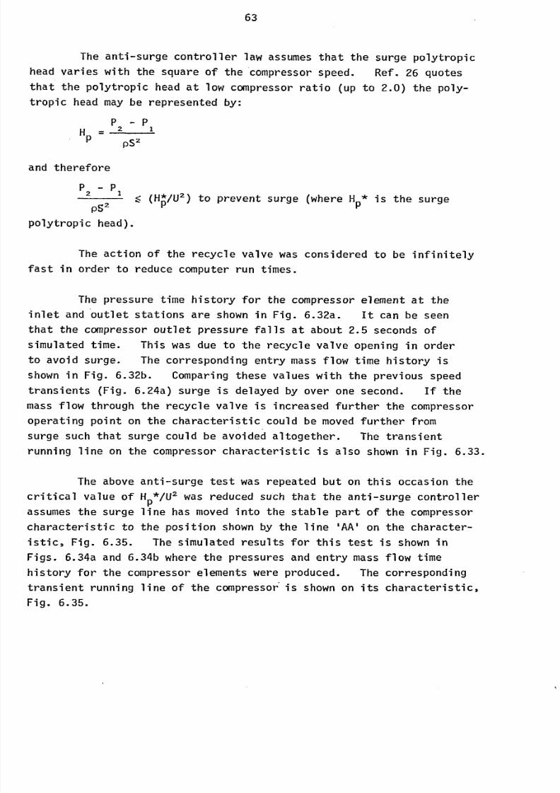
8/6/2019 A. M. Y. Razak Thesis 1984
http://slidepdf.com/reader/full/a-m-y-razak-thesis-1984 77/181
63
The anti-surge controller law assumes that the surge polytropic
head varies with the square of the compressor speed. Ref. 26 quotes
that the polytropic head at low compressor ratio (up to 2.0) the poly-
tropic headmay
berepresented
by:
p-p
HP2p
S2
and therefore
p2-
, C!2 . li pp4j
polytropic head).
The action of the recycle valve was considered to be infinitely
fast in order to reduce computer run times.
The pressure time history for the compressor element at the
inlet and outlet stations are shown in Fig. 6.32a. It can be seen
that the compressor outlet pressure falls at about 2.5 seconds ofsimulated time. This was due to the recycle valve opening in order
to avoid surge. The corresponding entry mass flow time history is
shown in Fig. 6.32b. Comparing these values with the previous speed
transients (Fig. 6.24a) surge is delayed by over one second. If the
mass flow through the recycle valve is increased further the compressor
operating point on the characteristic could be moved further from
surge such that surge could be avoided altogether. The transient
running line on the compressor characteristic is also shown in Fig. 6.33.
The above anti-surge test was repeated but on this occasion the
critical value of HPIUI was reduced such that the anti-surge controller
assumes the surge line has moved into the stable part of the compressor
characteristic to the position shown by the line 'AA' on the character-
istic, Fig. 6.35. The simulated results for this test is shown in
Figs. 6.34a and 6.34b where the pressures and entry mass flow time
history for the compressor elements were produced. The corresponding
transient running line of the compressor is shown on its characteristic,
Fig. 6.35.
,< (Hn-/u-) to prevent surge (where Hnw is the surger
8/6/2019 A. M. Y. Razak Thesis 1984
http://slidepdf.com/reader/full/a-m-y-razak-thesis-1984 78/181
8/6/2019 A. M. Y. Razak Thesis 1984
http://slidepdf.com/reader/full/a-m-y-razak-thesis-1984 79/181
65
the compressor outlet pressure falls off to a larger degree when compared
with the case when no non-return valves were present in the downstream
duct work. This was due to the additional pressure loss incurred
by thepresence of
thesenon-return valves.
Thecorresponding
transient
running line is shown in Fig. 6.37.
It can be seen in Figs. 6.36 and 6.3-7 that-the sudden surge
problem is (see section 6.22) not apparent and during this simulation the
downstream non-return valve did not operate. The pressure losses quoted
by the valve manufacturers are generally the maximum oss in order to
satisfy guarantee requirements. However, such valves may-have lower
pressure losses and the effect of lower pressure losses will be
considered later in section 6.27.
6.24 Effect of Active DownstreamNon-Return Valves on Compressor Surge
The above defined speed transient was again introduced. At
the time the speed transient was introduced (i. e. after 0.02 seconds
of steady state running), the pressure downstream of the last down-stream non-return valve was instantaneously increased by NOabove its
initial value, and maintained for 0.1 seconds of simulated time. This
increase in pressure was sufficient to close the downstream non-return
valves.
The pressures across the compressor element and the entry mass
flow time history is shown in Figs. 6.38a and 6.38b respectively.
Examining the compressor entry mass flow time history, Fig. 6.38b, it
can be seen that surge occurs quite quickly, furthermore the compressor
surges in approximately 0.075 seconds. The anti-surge recycle valve
having a stroke time of some 10 seconds will be unable to cope with
such fast transients. This condition is very similar to that observed
in the gas transmission station where such a sudden surge condition
occurs. This surge condition is produced by the throttling of the
gas flow due to the closure of the downstream non-return valves.
The non-return valve movements in the downstream discharge line
are shown in Figs. 6.39a and 6.39b respectively. The pressure difference
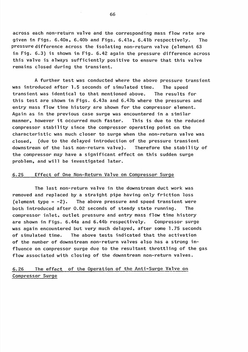
8/6/2019 A. M. Y. Razak Thesis 1984
http://slidepdf.com/reader/full/a-m-y-razak-thesis-1984 80/181
66
across each non-return valve and the corresponding mass flow rate are
given in Figs. 6.40a, 6.40b and Figs. 6.41a, 6.41b respectively. The
pressure difference across the isolating non-return valve (element 63in Fig. 6.3) is shown in Fig. 6.42 again the pressure difference across
this valve is always sufficiently positive to ensure that this valve
remains closed during the transient.
A further test was conducted where the above pressure transient
was introduced after 1.5 seconds of simulated time. The speed
transient was identical to that mentioned above. The results for
this test are shown in Figs. 6.43a and 6.43b where the pressures and
entry mass flow time history are shown for the compressor element.
Again as in the previous case surge was encountered in a similar
manner, however it occurred much faster. This is due to the reduced
compressor stability since the compressor operating point on the
characteristic was much closer to surge when the non-return valve was
closed, (due to the delayed introduction of the pressure transient
downstream of the last non-return valve). Therefore the stability of
the compressor may have a significant effect on this sudden surge
problem, and will be investigated later.
6.25 Effect of One Non-Return Valve on Compressor Surge
The last non-return valve in the downstream duct work was
removed and replaced by a straight pipehaving
onlyfriction loss
(element type = -2). The above pressure and speed transient were
both introduced after 0.02 seconds of steady state running. The
compressor inlet, outlet pressure and entry mass flow time history
are shown in Figs. 6.44a and 6.44b respectively. Compressor surge
was again encountered but very much delayed, after some 1.75 seconds
of simulated time. The above tests indicated that the activation
of the number of downstream non-return valves also has a strong in-
fluence on compressor surge due to the resultant throttling of the gas
flow associated with closing of the downstream non-return valves.
6.26 The effect of the Operation of the Anti-Surge Valve on
Compressor Surge
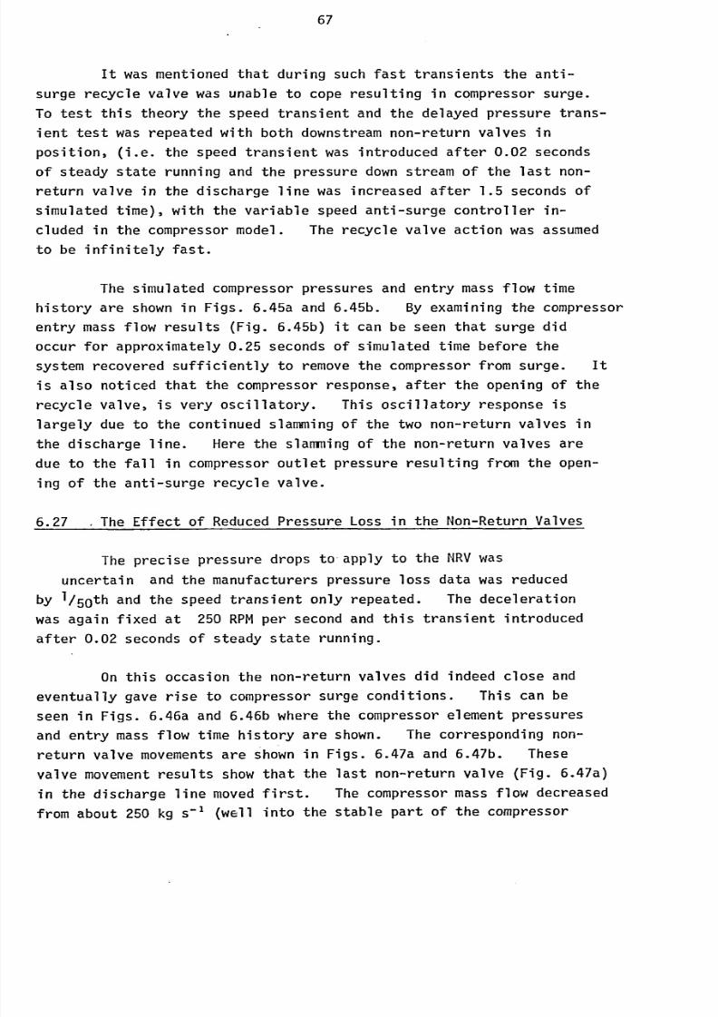
8/6/2019 A. M. Y. Razak Thesis 1984
http://slidepdf.com/reader/full/a-m-y-razak-thesis-1984 81/181
67
It was mentioned that during such fast transients the anti-
surge recycle valve was unable to cope resulting in compressor surge.
To test this theory the speed transient and the delayed pressure trans-
ient test was repeated with both downstream non-return valvesin
position, (i. e. the speed transient was introduced after 0.02 seconds
of steady state running and the pressure down stream of the last non-
return valve in the discharge line was increased after 1.5 seconds of
simulated time), with the variable speed anti-surge controller in-
cluded in the compressor model. The recycle valve action was assumed
to be infinitely fast.
The simulated compressor pressures and entry mass flow time
history are shown in Figs. 6.45a and 6.45b. By examining the compressor
entry mass flow results (Fig. 6.45b) it can be seen that surge did
occur for approximately 0.25 seconds of simulated time before the
system recovered sufficiently to remove the compressor from surge. it
is also noticed that the compressor response, after the opening of the
recycle valve, is very oscillatory. This oscillatory response is
largely due to the continued slamming of the two non-return valves inthe discharge line. Here the slamming of the non-return valves are
due to the fall in compressor outlet pressure resulting from the open-
ing of the anti-surge recycle valve.
6.27.
The Effect of Reduced Pressure Loss in the Non-Return Valves
Theprecise
pressure drops to apply to the NRVwas
uncertain and the manufacturers pressure loss data was reduced
by 1/50th and the speed transient only repeated. The deceleration
was again fixed at 250 RPMper second and this transient introduced
after 0.02 seconds of steady state running.
On this occasion the non-return valves did indeed close and
eventually gave rise to compressor surge conditions. This can be
seen in Figs. 6.46a and 6.46b where the compressor element pressures
and entry mass flow time history are shown. The corresponding non-
return valve movementsare shown in Figs. 6.47a and 6.47b. These
valve movement results show that the last non-return valve (Fig. 6.47a)
in the discharge line moved first. The compressor mass flow decreased
from about 250 kg s-1 (wEll into the stable part of the compressor
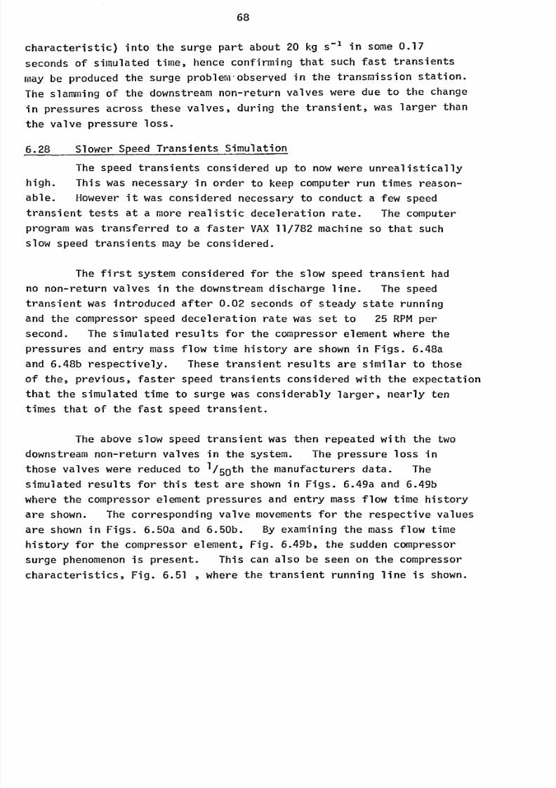
8/6/2019 A. M. Y. Razak Thesis 1984
http://slidepdf.com/reader/full/a-m-y-razak-thesis-1984 82/181
68
characteristic) into the surge part about 20 kg s-1 in some0.17
seconds of simulated time, hence confirming that such fast transients
may be produced the surge problem-observed in the transmission station.
The slamming of the downstream non-return valves were due to the change
in pressures across these valves, during the transient, was larger than
the valve pressure loss.
6.28 Slower Speed Transients Simulation
The speed transients considered up to now were unrealistically
high. This was necessary in order to keep computer run times reason-
able. However it was considered necessary to conduct a few speed
transient testsat a more realistic
decelerationrate.
Thecomputer
program was transferred to a faster VAX11/782 machine so that such
slow speed transients may be considered.
The first system considered for the slow speed transient had
no non-return valves in the downstream discharge line. The speed
transient was introduced after 0.02 seconds of steady state running
and the compressor speed deceleration rate was set to 25 RPMper
second. The simulated results for the compressor element where the
pressures and entry mass flow time history are shown in Figs. 6.48a
and 6.48b respectively. These transient results are similar to those
of the, previous, faster speed transients considered with the expectation
that the simulated time to surge was considerably larger, nearly ten
times that of the fast speed transient.
The above slow speed transient was then repeated with the twodownstream non-return valves in the system. The pressure loss in
those valves were reduced to 1150th the manufacturers data. The
simulated results for this test are shown in Figs. 6.49a and 6.49b
where the compressor element pressures and entry mass flow time history
are shown. The corresponding valve movementsfor the respective values
are shown in Figs. 6.50a and 6.50b. By examining the mass flow time
history for the compressor element, Fig. 6.49b, the sudden compressor
surge phenomenon s present. This can also be seen on the compressor
characteristics, Fig. 6.51, where the transient running line is shown.
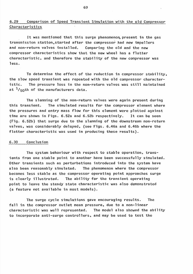
8/6/2019 A. M. Y. Razak Thesis 1984
http://slidepdf.com/reader/full/a-m-y-razak-thesis-1984 83/181
8/6/2019 A. M. Y. Razak Thesis 1984
http://slidepdf.com/reader/full/a-m-y-razak-thesis-1984 84/181
70
efficiency of control systems used in process plants.
The development of the boundary condition for use in an "in
finite" system appear to have been very successful. The infinite
boundary condition highlights compressor surge problems during shut
down.
Increasing the number of elements downstream tends to help
avoid surge conditions and is mainly due to the increase in loss in
the system. The double and single discharge header was also simulated,
and the results indicate that the double discharge system is likely toreach compressor surge before the single discharge system. This is
in line with experience in the real system.
All the tests conducted on the non-return valve 3, (fig. 6.23),
show that the pressure difference across this valve is always large
enough to ensure that this element remains inactive (closed). The
necessary pressure difference required to open this valve is unlikely
to be attained under operating conditions simulated in this thesis.
The case when the steeper characteristic was used surge occurred
but somewhat delayed. The non-return valve did slam in this case
too. The surge resulted due to the operation of these downstream non-
return valves where the gas flow through these valves are throttled
when the valves close.
The slamming of these downstream non-return valves appears to
be the real cause of the problem since the operation of these valves
throttle the compressor discharge gas making the compressor surge
prone. A reduction of the number of non-return valves will help
the system as was illustrated in figs. 6.44a and 6.44b where only one
of the downstream return valves was present (the non-return valve
closest to the compressorin the discharge line), due to the
reducedthrottling effect. However, increasing the pressure loss on each
valve will prevent the valve slamming but the system will operates
less efficiently.
8/6/2019 A. M. Y. Razak Thesis 1984
http://slidepdf.com/reader/full/a-m-y-razak-thesis-1984 85/181
71
A system that may have such an arrangement having only one
non-return valve in the discharge line irrespective of the number of
compressor units present in the station is shown in fig. 6.53. The
limitation of such a system is that only parallel operation of the
compressor units is possible. However this transmission station has
never used the compressor units in series. Furthermore, when any
one unit is operational, (the proposed system Fig. 6.53), the gas
has to flow through only one non-return valve unlike two valves with
the current system. This will result in lower pressure loss hence
making the station more efficient. Alternatively the pressure loss
inthe non-return valve may
be increasedsufficiently to prevent the
non-return valve slamming hence over coming the surge problem.
8/6/2019 A. M. Y. Razak Thesis 1984
http://slidepdf.com/reader/full/a-m-y-razak-thesis-1984 86/181
72
CHAPTER
7.0 DISCUSSIONND SUGGESTIONORFURTHER ORK
Increasing the losses in the gas transmission system will result
in a steeper transient running line on the compressor characteristic.
However,surge encountered
due toa relatively
flat transientrunning
line may be satisfactorily overcome by the anti-surge recycle valve
since this transient is relatively slow. The throttling of the gas
flow in the downstream discharge line, due to the slamming of the non-
return valve, introduce rapid transients, and the recycle valve is un-
able to cope resulting in compressor surge operation. Reducing the
number of non-return valves in the discharge line helps this surge
problem due to the reduction of the throttling effect and therefore
giving the recycle valve a better chance to cope.
7.1 Non-Return Valve
In order to simulate the case when these downstream non-return
valves may operate during a speed transient it was necessary to reduce
the pressure losses in these valves. The pressure loss was reduced
in steps Of1125th
of the valve manufacturers data until the valvemovements occurred (i. e. a pressure loss of 1/100th of the pressure
loss data was necessary in order to obtain the valve movement). A
better estimation of the pressure loss may be obtained by undertaking
an experimental investigation on these non-return valves. Further-
more the valve mass and spring stiffness data were not readily
available and these values were obtained by approximate calculation
of valve volume and density of the material. The reasonable valve
stiffness was. (225 Nm-') assumed. The above information from the
valve manufacturer will enable a more accurate simulation.
8/6/2019 A. M. Y. Razak Thesis 1984
http://slidepdf.com/reader/full/a-m-y-razak-thesis-1984 87/181
73
7.2 Boundary Condition
The impedance boundary condition requires that the pressuresupstream of the system boundaries (i. e. upstream of element 1 and
downstream of element 48 in fig. 6.4) must be largely constant. This
condition satisfies the assumption that the acoustic impedance upstream
of elements 1 and 2 (fig. 6.4) are equal, and similarly downstream of
elements 48 and 47 are also equal. However, the pressures in the
pipeline may vary considerably as the pipeline serves a secondary
function of gas storage.
The satisfactory manner to account for such pressure variations
is to model the pipeline all way down to the consumer. Should such a
simulation be attempted, the number of elements may run into tens of
thousands and the computer run times of such a simulation will be
prohibitively high. If a simulation accounting for such pipeline
pressure variation were required a reasonable approximation may be
to use the nozzle relations discussed in Chapter 3. The plenum
pressure to which the nozzle exhausts to may be determined by performing
an instantaneous mass balance of a given control volume, VP, down-
stream of the system considered. Using the value of the mass, m,
within this control volume the approximate instantaneous plenum
Pressure, Ps, may be determined via the equation of state psVP=mRts*
A similar method may be used to determine the system entry pressure.
7.3 Intercoolers
Intercoolers are commonoccurrence in process plants.
Detailed analysis of this type of element has yet to be performed.
It is expected that such an element may be modelled similar to that
of a duct with loss type element discussed in Chapter 3, and the exit
temperature determined from the intercooler effectiveness equation.
7.4 Computer Run Times
A significant problem uncovered during this project has been
the very long computer program executing times, particularly when many
elements are involved in defining a system. Although using a powerful
8/6/2019 A. M. Y. Razak Thesis 1984
http://slidepdf.com/reader/full/a-m-y-razak-thesis-1984 88/181
74
computer and a faster integrating technique helps matters, a subý
stantial reduction in executing times may be obtained by using parallel
or array process i ng
7.5 Additional Application for the Technique
The application of the model may be considered for many systems
where one-dimensional flow analysis is required. There are instances
where two dimensional flow considerations are required. One such
example is the effect of after-burning, in low-by pass ratio turbo-fanengines, on low pressure compressor surge.
The problem may be attacked by dividing the low pressure
compressor into two parallel systems along the by pass splitter
axially. The flows between the compressor stages and at the splitter
may be patched using the patch procedure discussed in Chapter 6.
The steady state compressor characteristic for the two systems is
required, (i. e. below and above the splitter line), in order to
determine the required body force terms. The respective system entry
pressures may be found by studying the radial equilibrium criteria
used (i. e. free vortex or constant reaction etc. ).
The disadvantage of the above method is that flows crossing
the systems within the stages are not accounted for. However, the
radial pressure gradient that exists within the compressor stage will
ensure that most of the flow crossing the system dividing line will
occur within stages. lience.reducing any error due to the assumption that
no flows crossing the dividing line with the stage.
8/6/2019 A. M. Y. Razak Thesis 1984
http://slidepdf.com/reader/full/a-m-y-razak-thesis-1984 89/181
75
CHAPTER
8.0 CONCLUSIONS
This project, in the main, has been concerned with the
application of a mathematical model which can simulate process plant
system transients, in particular centrifugal compressor transients
used in natural gas transmission systems. After the development ofthe model it was considered necessary to undertake an experimental
validation programme.
8.1 The Model
The derivation of the mathematical model has involved several
assumptions. Firstly, the one-dimensional flow assumption, although
this appears to be a drastic simplification of the complex flow
structure known to exit it does not appear to be a limiting factor as
proven by the results obtained in this study. Furthermore such
assumptions have been made in many other models and good results have
been obtained. The model employed here is considered to be much
easier to apply compared with those described in Ref. 8, and where
again momentum nd continuity equations were used in the derivation.
Secondly the assumption of low Mach number at the boundaries
of the discretisation process (less than 0.3) implies that the element
boundaries should be chosen to comply with this requirement. Thirdly,
the justification for neglecting the dynamic effects of the energy
equation is simply that results are little effected and the computational
effort is much reduced (Ref. 10,11). Finally, the lumped parameter and
the quasi-steady state assumptions impose frequency limitations on themodel. These limitations are not serious so long as care is taken
and the element length is much less than the wave length of the flow
perturbations.
8/6/2019 A. M. Y. Razak Thesis 1984
http://slidepdf.com/reader/full/a-m-y-razak-thesis-1984 90/181
76
General application rules for the geometric distribution of
element have been formulated. The first, relating element length
with a frequency parameter, is based upon the workof
Elder (Ref.
and is derived from the comparison of the lumped and true partial
differential solutions. The critical frequency parameter obtained
from this study is set such that the error between these two solutions
is small (less than 5%). The second criteria, namely approximately
equal volumes, is necessary to ensure that the elements will interact
with each other to a larger extent.
8.2_.
Experimental Validation
The mathematical model was validated using transient data
obtained from a small centrifugal compressor of a turbo-charger. The
general agreement between the simulated and experimental results is
very good. The slight discrepancies are very largely attributed to the
inaccuracies in the representation of the poppet valve action. The
surge validation test gave equally encouraging results.
It is not reasonable to expect a model of this type to simulate
full compressor surge cycles without accurate knowledge of the post
surge compressor characteristic. If such characteristics are available
it is thought that the model is capable of simulating complete surge
cycles.
8.3 Simulation of Natural Gas Transmission System
The behaviour of the natural gas transmission system during
transient changes between two stable operating conditions has success-
fully been simulated. The system response to perturbations introduced
into the system have also been reasonably simulated. The reduced
stability of the compressor when surge is approached has been clearly
illustrated.
Compressor surge simulation gave encouraging results. The
fall of the mean compressor outlet pressure, due to the non-linear
nature of the compressor characteristic near surge, was well represented.
8/6/2019 A. M. Y. Razak Thesis 1984
http://slidepdf.com/reader/full/a-m-y-razak-thesis-1984 91/181
77
The ability to test the efficiency of anti-surge control systems is
also possible. Pre surge and post surge simulation has also been
performed (i. e. the case when the anti-surge recycle are opened after
the compressor had surged).
The development of the "infinite volume" boundary condition
appear to be successful and this boundary condition indicated compressor
surge problems during shut down. The single and double discharge
operation simulation showed the compressor surge delayed when the
single discharge system was operational. This was due to the higher
velocities in the discharge pipe during single discharge operation
resulting in higher pipe pressure loss which tends to delay surge.
The model was also successful in highlighting compressor surge
problems associated with the operation of the downstream discharge
line non-return valves. The activation of these valves throttles
the gas flow in the discharge line resulting in compressor surge.
This throttlingeffect
introducesrapid
transients into thesystem
to
make the recycle anti-surge valve ineffective. Even when the re-
cycle valve time constant was put to zero compressor surge occurred.
This sudden surge phenomenon s present in the plant and apparently
the non-return valves are the cause of this surge problem.
The operation of these downstream non-return valves could be
prevented if the pressure loss associated with these valves were in-
creased, and therefore overcoming the surge problem. However, this
will result in the plant becoming inefficient and a higher operating
cost. The model was used to study the effect of one non-return valve
in the down stream discharge line. This study indicated compressor
surge to be delayed, due to the reduced effect of the throttling of
the gas flow in the discharge line. Since only one non-return valve
is present the pressure loss may be increased in this valve without
suffering a significant loss in plant efficiency hence help overcomethis unexpected compressor surge problem.
8/6/2019 A. M. Y. Razak Thesis 1984
http://slidepdf.com/reader/full/a-m-y-razak-thesis-1984 92/181
78
The steeper compressor characteristic also gave surge conditions
although delayed comparedwith the case of the flatter characteristic.
Howeverstable
thecharacteristic
ismade, sufficient
throttling of
the downstream gas flow (due to the activation of the non-return valves)
will give surge condition.
8.4 Numerical Method
Single step methods are generally self starting and the
estimation of the integration error is relatively easy. Of the many
single step methods available, that of Runge-Kutter-14erson s very
efficient. To this effect the Runge-Kutta-Merson method was used to
solve the non-linear differential equations derived in Chapter 2.
Another efficient method that is becoming increasingly popular is
the Runge-Kutta-Feh1berg method.
Multi-step methods.are computationally more efficient but they
have the disadvantages of not being self starting and the estimation
of the integration error is awkward. A multi-step method that is
stable, accurate and particularly recommendedor so called stiff
equations is Gears method. Other multi-step methods worth considering
are Adam-Moulton and Hammingsmethods.
8.5 Numerical Instabilities
Numerical instabilities were incurred where the volumes of
elements in the vicinity of branches and butts (or stub) are very
similar. These instabilities are apparently due to flows pulsating
in branches (and butts) exciting oscillations in the main stream
elements in the neighbourhood.
It was found that such instabilities may be avoided if the
element volumes near branches (and butts) were staggered. A± 10%
change in these element volumes are possible without introducing a

8/6/2019 A. M. Y. Razak Thesis 1984
http://slidepdf.com/reader/full/a-m-y-razak-thesis-1984 93/181
79
significant error in the simulation. Another approach to these
instabilities is to increase the friction force in elements in the
neighbourhood ofbranches (and butts)
sothat these
oscillations maybe dampedto a larger degree. However, this may result in an un-
realistic pressure loss in these elements. Apart from these problems
the model proved relatively simple to use.
8/6/2019 A. M. Y. Razak Thesis 1984
http://slidepdf.com/reader/full/a-m-y-razak-thesis-1984 94/181
80
CHAPTER
9.0 SUMMARYF CONCLUSIONS
A mathematical model capable of simulating centrifugal compressor
transient performance within a process system has been developed and
implemented in a Fortran computer program. The model is applicable
to any type of process plant, and can deal with non-ideal gases. The
analysis is limited to one dimensional flow consideration. A com-
parison of simulated and measured compressor transients has shown that:
(1) Simulation of transients between stable operating points has
been performed with reasonable accuracy.
(2) Satisfactory compressor surge simulation has been performed
in terms of variable time history.
(3) The computer code has been prepared in a modular fashion to
permit different studies to be easily made. In addition to
this project described here, multi-stage axial and centrifugal
compressors may be considered.
The model was successfully applied to a natural gas transmissionsystem, having operational problems associated with plant dynamics.
The model highlighted compressor surge problems due to the interaction
of the compressor with plant controls. Through these studies a
possible solution to the compressor surge problem was suggested.
The model has the potential to be used as a design tool to
study plant dynamic problems or improving the dynamic performance of
existing plants. Another application for the model is the accident
investigation of process plants.
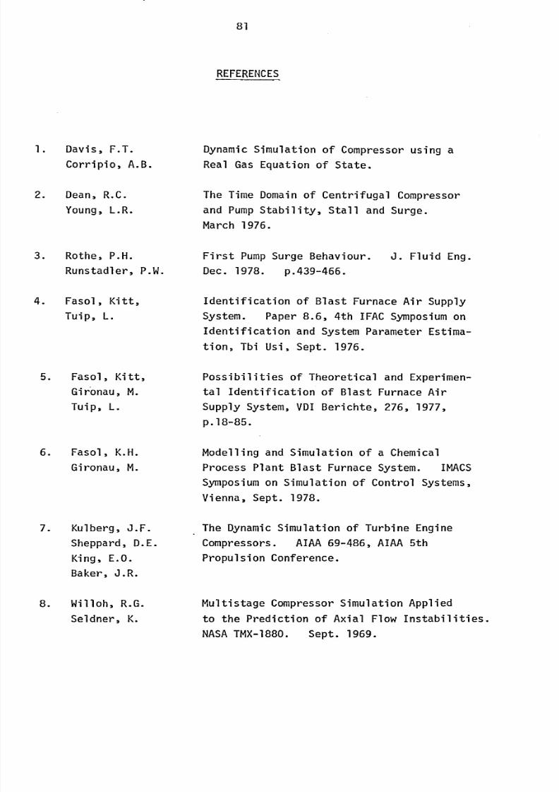
8/6/2019 A. M. Y. Razak Thesis 1984
http://slidepdf.com/reader/full/a-m-y-razak-thesis-1984 95/181
81
REFERENCES
Davis, F.T.
Corripio, A.B.
Dean, R. C.
Young, L. R.
3. Rothe, P.H.
Runstadler, P. W.
4. Fasol, Kitt,
Tuip, L.
5. Fasol, Kitt,
Gironau, M.
Tuip, L.
6. Fasol, K.H.
Gironau, M.
7. Kulberg, J. F.
Sheppard, D. E.
King, E. O.
Baker, J. R.
8. Willoh, R. G.
Seldner, K.
Dynamic Simulation of Compressor using a
Real Gas Equation of State.
The Time Domain of Centrifugal Compressor
and PumpStability, Stall and Surge.
March 1976.
First PumpSurge Behaviour. J. Fluid Eng.
Dec. 1978. p. 439-466.
Identification of Blast Furnace Air Supply
System. Paper 8.6,4th IFAC Symposiumon
Identification and System Parameter Estima-tion, Tbi Usi, Sept. 1976.
Possibilities of Theoretical and Experimen-
tal Identification of Blast Furnace Air
Supply System, VDI Berichte, 276,1977,
p. 18-85.
Modelling and Simulation of a Chemical
Process Plant Blast Furnace System. IMACS
Symposiumon Simulation of Control Systems,
Vienna, Sept. 1978.
The Dynamic Simulation of Turbine Engine
Compressors. AIAA 69-486, AIAA 5th
Propulsion Conference.
Multistage Compressor Simulation Applied
to the Prediction of Axial Flow Instabilities.
NASATMX-1880. Sept. 1969.
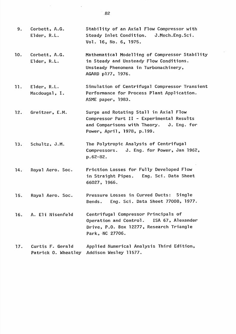
8/6/2019 A. M. Y. Razak Thesis 1984
http://slidepdf.com/reader/full/a-m-y-razak-thesis-1984 96/181
8/6/2019 A. M. Y. Razak Thesis 1984
http://slidepdf.com/reader/full/a-m-y-razak-thesis-1984 97/181
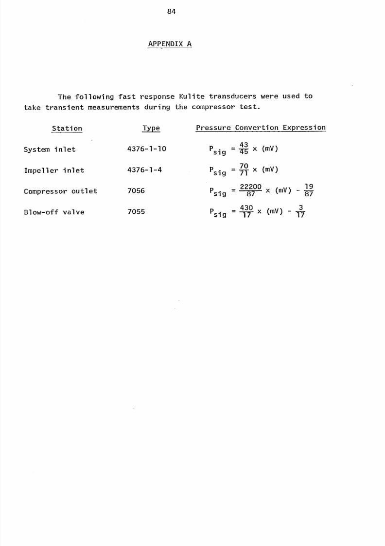
8/6/2019 A. M. Y. Razak Thesis 1984
http://slidepdf.com/reader/full/a-m-y-razak-thesis-1984 98/181
84
APPENDIX
The following fast response Kulite transducers were used to
take transient measurements during the compressor test.
Stati on Type Pressure Convertion Expression
System inlet 4376-1-10 P
43
` 475x (MVSig
Impeller inlet 4376-1-4 P0Sig
L71x (mV)
Compressor outlet 7056 P22200 19
Sig 87 x (mV) - 87
Blow-off valve 7055 PA30
x (mV) _3Sig 17 17
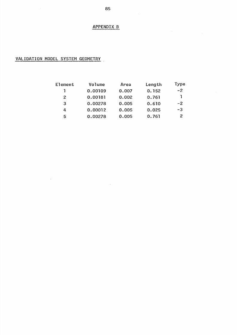
8/6/2019 A. M. Y. Razak Thesis 1984
http://slidepdf.com/reader/full/a-m-y-razak-thesis-1984 99/181
85
APPENDIX
VALIDATIONMODEL YSTEMGEOMETRY
Element Volume Area Length Type
10.00109 0.007 0.152 -2
2 0.00181 0.002 0.761 1
3 0.00278 0.005 0.610 -2
4 0.00012 0.005 0.025 -3
5 0.00278 0.005 0.761 2
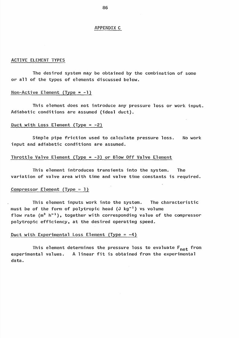
8/6/2019 A. M. Y. Razak Thesis 1984
http://slidepdf.com/reader/full/a-m-y-razak-thesis-1984 100/181
86
APPENDIX
ACTIVE ELEMENTYPES
The desired system may be obtained by the combination of some
or all of the types of elements discussed below.
Non-Active Element (Type = -1)
This element does not introduce any pressure loss or work input.
Adiabatic conditions are assumed (ideal duct).
Duct with Loss Element (Type = -2)
Simple pipe friction used to calculate pressure loss. No work
input and adiabatic conditions are assumed.
Throttle Valve Element (Type = -3) or Blow Off Valve Element
This element introduces transients into the system. The
variation of valve area with time and valve time constants is required.
Compressor Element (Type = 1)
This element inputs work into the system. The characteristic
must be of the form of polytropic head (J kg-') vs volume
flow rate (m' h-'), together with corresponding value of the compressor
polytropic efficiency, at the desired operating speed.
Duct with ExperimentalLoss
Element(Type
= -4)
This element determines the pressure loss to evaluate Fnet from
experimental values. A linear fit is obtained from the experimental
data.
8/6/2019 A. M. Y. Razak Thesis 1984
http://slidepdf.com/reader/full/a-m-y-razak-thesis-1984 101/181
87
Therefore
AP =A *slope+ constant
Diffuser Element (Type = -5)
This element is used to represent an expanding duct.
Nozzle Element (Type = -6)
As the name suggests this element represents a converging duct.
Valve Element (Type = -7)
A recycle valve is represented by this element. It may be
used as an isolating valve or a means of introducing a transient into
the system. The valve area variation with time and the valve stroke
time isrequired.
Bend Element (Type = -8)_
This element is used to represent a right angle bend.
Branch Element (Type = -9)
Combining and dividing flows are represented by this element.
This element also patches sub-system when parallel systems are considered.
Non-Return Valve Element (Type =6 and 7)
This element represents a valve that is operated by the pressure
difference across it. If TYPE=6 it is assumed the valve is initially
closed. When TYPE=7 the valve is initially opened.
8/6/2019 A. M. Y. Razak Thesis 1984
http://slidepdf.com/reader/full/a-m-y-razak-thesis-1984 102/181
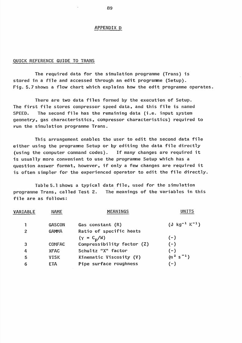
8/6/2019 A. M. Y. Razak Thesis 1984
http://slidepdf.com/reader/full/a-m-y-razak-thesis-1984 103/181
89
APPENDIXD
QUICKREFERENCEUIDETO TRANS
The required data for the simulation programme (Trans) is
stored in a file and accessed through an edit programme (Setup).
Fig. 5.7shows a flow chart which explains how the edit programme operates.
There are two data files formed by the execution of Setup.
The first file stores compressor speed data, and this file is named
SPEED. The second file has the remaining data (i. e. input system
geometry, gas characteristics, compressor characteristics) required to
run the simulation programmeTrans.
This arrangement enables the user to edit the second data file
either using the programmeSetup or by editing the data file directly
(using the computer command odes). If many changes are required it
is usually more convenient to use the programmeSetup which has a
question answer format, however, if only a few changes are required it
is often simpler for the experienced operator to edit the file directly.
Table 5.1 shows a typical data file, used for the simulation
programmeTrans, called Test 2. The meanings of the variables in thisfile are as follows:
VARIABLE NAME MEANINGS UNITS
I GASCON Gas constant (R)
2 GAMMA Ratio of specific heats
(Y=Cp
/W)
3 COMFAC Compressibility factor (Z)
4 XFAC Schultz 'T' factor
5 VISK Kinematic Viscosity (V)
6 ETA Pipe surface roughness
(J kg-' K-1)
HHHW
H
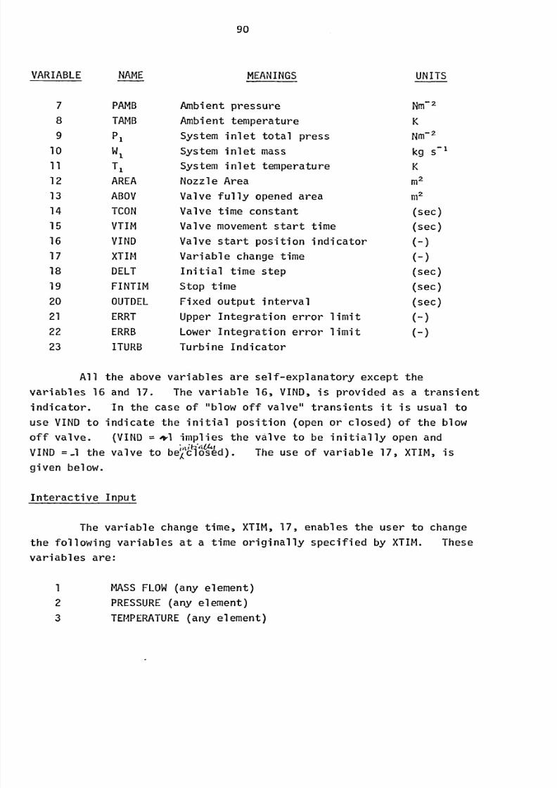
8/6/2019 A. M. Y. Razak Thesis 1984
http://slidepdf.com/reader/full/a-m-y-razak-thesis-1984 104/181

8/6/2019 A. M. Y. Razak Thesis 1984
http://slidepdf.com/reader/full/a-m-y-razak-thesis-1984 105/181
91
5
6
7
GAMMAy)
GASCONSTANTR)
COMFACZ)
XFAC(X)
Furthermore, future variable changes are possible without altering
the previously chosen value of XTIM (i. e. XTIM may be altered through
the simulating program (Trans), when the accumulated time is equal to
or greater than the initial value of XTIM).
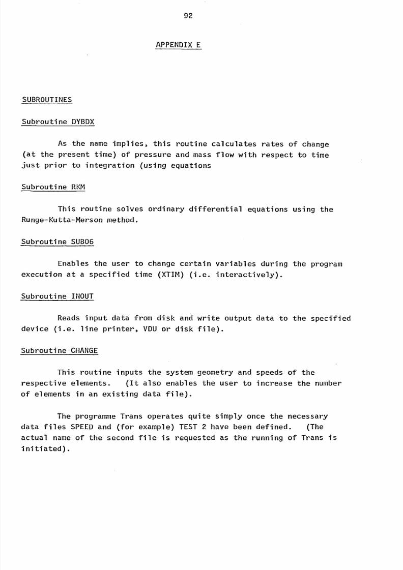
8/6/2019 A. M. Y. Razak Thesis 1984
http://slidepdf.com/reader/full/a-m-y-razak-thesis-1984 106/181
92
APPENDIX
SUBROUTINES
Subroutine DYBDX
As the nameimplies, this routine calculates rates of change
(at thepresent
time)of pressure and mass flow with respect to time
just prior to integration (using equations
Subroutine RKM
This routine solves ordinary differential equations using the
Runge-Kutta-Merson method.
Subroutine SUB06
Enables the user to change certain variables during the program
execution at a specified time (XTIM) (i. e. interactively).
Subroutine INOUT
Reads input data from disk and write output data to the specifieddevice (i. e. line printer, VDUor disk file).
Subroutine CHANGE
This routine inputs the system geometry and speeds of the
respective elements. (It also enables the user to increase the number
of elements in an existing data file).
The programmeTrans operates quite simply once the necessary
data files SPEED nd (for example) TEST2 have been defined. (The
actual name of the second file is requested as the running of Trans is
initiated).

8/6/2019 A. M. Y. Razak Thesis 1984
http://slidepdf.com/reader/full/a-m-y-razak-thesis-1984 107/181
93
Both data files can be defined using the programmeSetup.
Running of this programmehas a question-answer system which is self
explanatory. The second file (for example TEST2) must be provided
for the successful operation of Trans but the file is only required if
the compressor shaft speed fluctuates.
Subroutine SUB01
This routine calls the subroutines defining the type of elements
present in the system (i. e. duct with loss, compressor, valves, etc
as discussed in Appendix A).
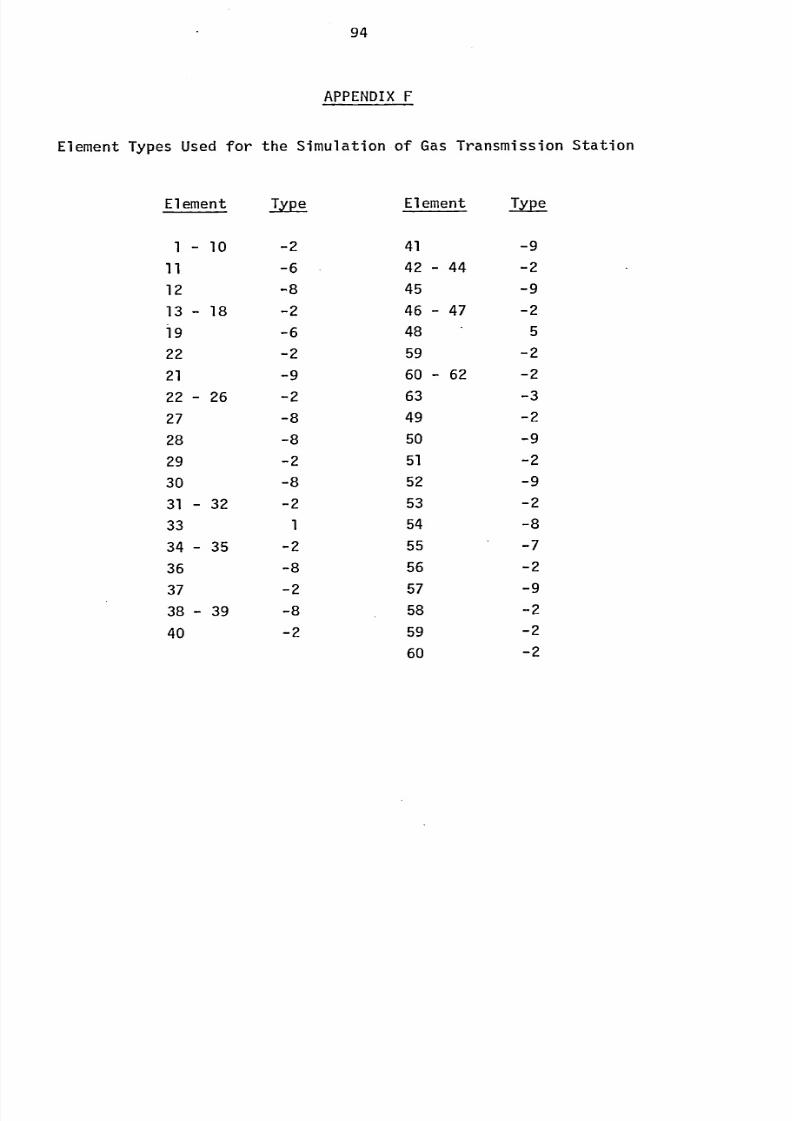
8/6/2019 A. M. Y. Razak Thesis 1984
http://slidepdf.com/reader/full/a-m-y-razak-thesis-1984 108/181
94
APPENDIX
Element Types Used for the Simulation ofGas Transmission Station
Element Type Element Type
1- 10 -2 41 -9
11 -6 42 - 44 -2
12 -8 45 -9
13 18 -2 46 - 47 -2
19 -648 5
22 -2 59 -2
21 -9 60 - 62 -2
22 26 -2 63 -3
27 -8 49 -2
28 -8 50 -9
29-2
51-2
30 -8 52 -9
31 - 32 -2 53 -2
33 1 54 -8
34 - 35 -2 55 -7
36 -8 56 -2
37 -2 57 -9
38 - 39 -8 58 -2
40 -2 59 -2
60 -2
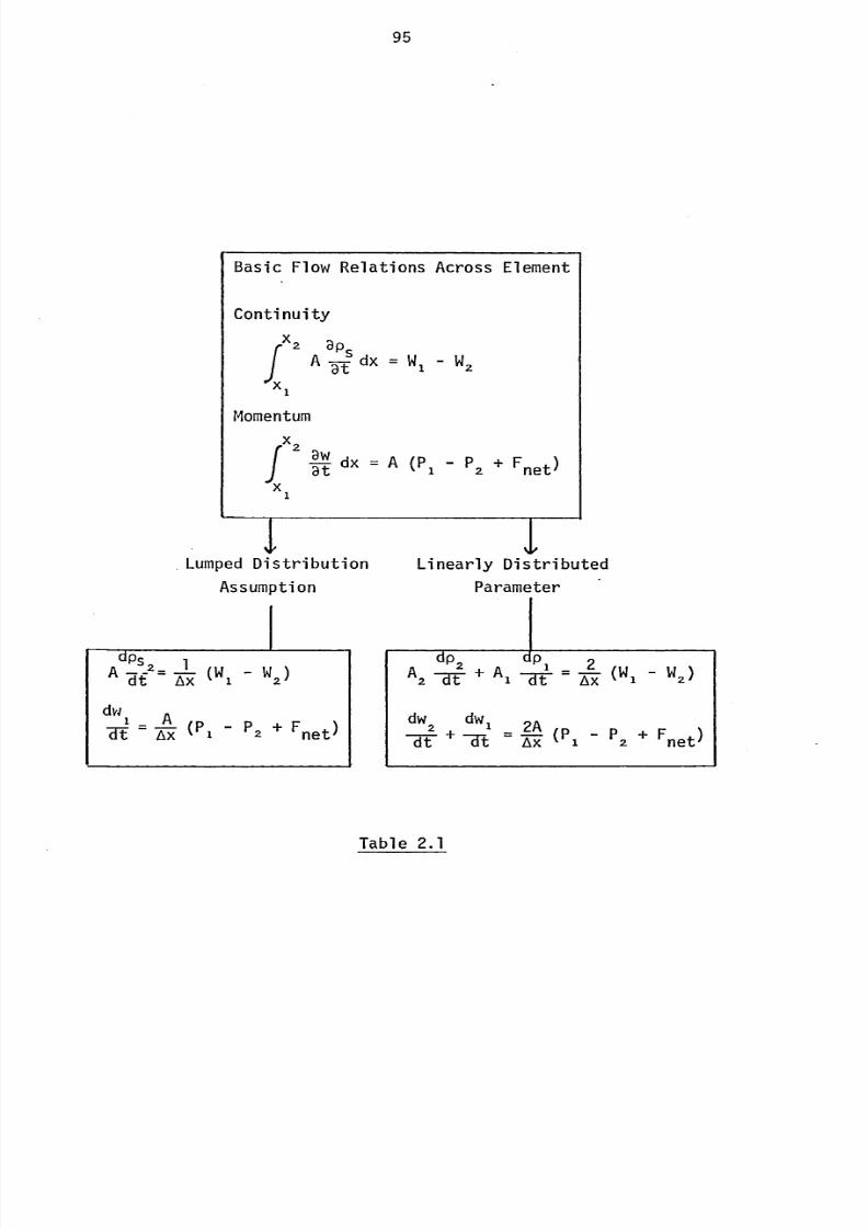
8/6/2019 A. M. Y. Razak Thesis 1984
http://slidepdf.com/reader/full/a-m-y-razak-thesis-1984 109/181
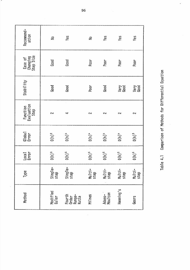
8/6/2019 A. M. Y. Razak Thesis 1984
http://slidepdf.com/reader/full/a-m-y-razak-thesis-1984 110/181
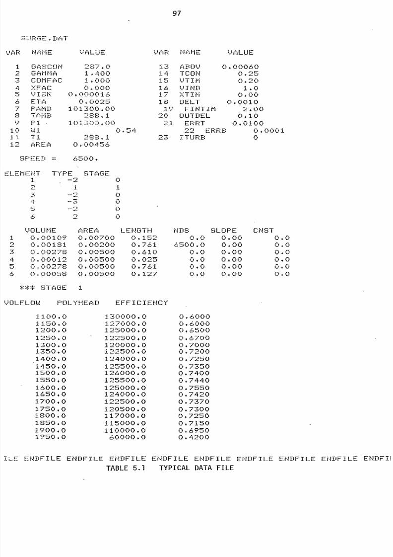
8/6/2019 A. M. Y. Razak Thesis 1984
http://slidepdf.com/reader/full/a-m-y-razak-thesis-1984 111/181
97
S, -E.Diý
VAR N: ME
DO2GAHHA
-1 COHFAC
Al XFAC
E Til)
PAMBTAMB
I
i. 2 iý'i Eit's
SF:,ý::: T-1 =:
.. - 1.. ý.
L I, E
1.400
4 Dol-I
cloo0,0 C-1.6
0 0025
1.0 13,0 A. 002 SEL. 1
1.Cl1 -3 -0, C.
0,54
0
6500.
TY PE ST()GE
-2 0
0
5 --2 0
4 7)tj -C.
VOLUME AREALENGTH1 0.00109 0.00700 0.152
2 0+00131 0.00200 04761
3 0.00278 0.00500 0010
4 0.00012 0.00500 0.025
5 OM278 0.00500 0.761
6 0.00058 0.00500 0.127
, ,wl.,_.
1-1S ` GE1.
VOL.FLOWI POLYHEAEI EFFICIENCY
1100.0 13000040
1150.0 127000.0
1200.0 125000.0
1250.0 122500+0
1300.0 120000.0
1350.0 122500.0
1400.0 124000.0
1450.0 125500.0
1500,0 126000*0
1550*0 125500+0
1600.0 125000.0
1650,0 124000.0
1700*0 122500.0
1750+0 120500.0
1800.0 117000.0
1850.0 11500040
1900.0 110000*01? 50.0 60000.0
WIR NI';MEVAL UEE
13 ABOV 0.00060
14TCON
0.2515 VTIM 0.20
16 VIND 1*017 XTIM 0.00
18 DELT 0.0010
19 FINTIM 2.0020 OUTDEL 0.10
21 ERRT 0.0100
22 ERRD 0.0001.23 1TURB 0
NDS SLOPE CNST. .. C. 0.00 C,.0
. '.500 0.00 0*
0.0 0. oc, 0. D
0.0 0400 0.0
0 0.00 C,i C.
0.0 0.00 0.0
0A000
0.60000* 6500
0* 6700
0* 70000.7200
0.7250
0.73500.7400
0.7440
0* 75500.7420
0.7370
0.73000* 7250
0.7150
0.69500.4200
ENDFILE ENEIFTLE ENDFILE EAEFIL. E ENDFILE EN111FILE EENDFILE E-NDFI'LiE ENDF11
TABLE 5.1 TYPICAL DATA FILE
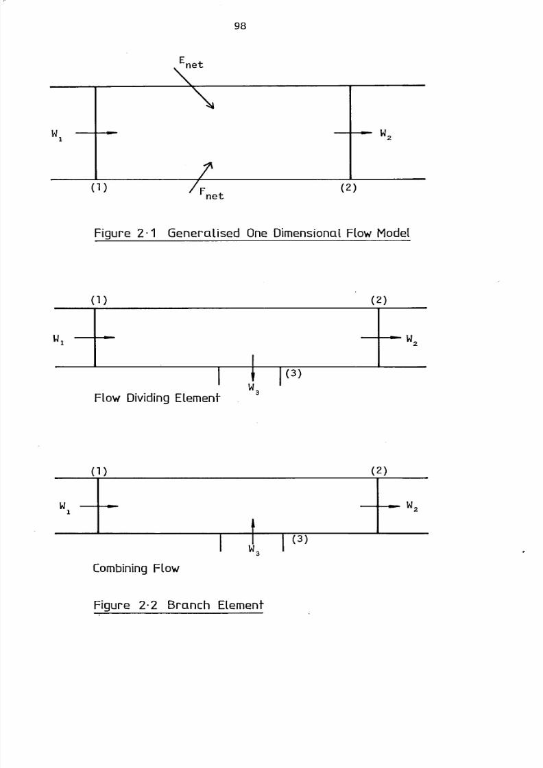
8/6/2019 A. M. Y. Razak Thesis 1984
http://slidepdf.com/reader/full/a-m-y-razak-thesis-1984 112/181
98
Wi
w
1
w3
I
I11w3
Figure2-1 Generalised OneDimensional lowMode[
(1)
I
Flow DividingEtement
(1)
Combiningow
(2)
(2)
w2
w2
Figure 2-2 Branch Element
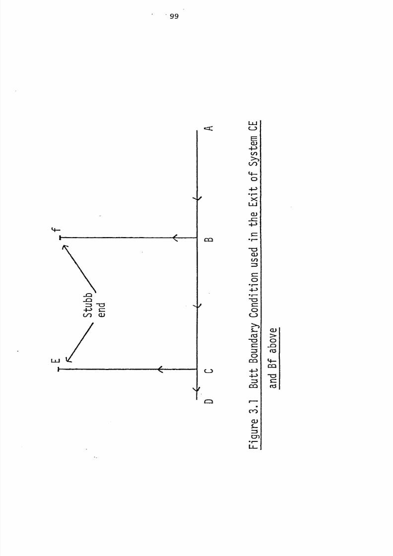
8/6/2019 A. M. Y. Razak Thesis 1984
http://slidepdf.com/reader/full/a-m-y-razak-thesis-1984 113/181
. 99
9-
Ld
k /
m
LLI
L-)
E-=(3)4J
V)
4-0
4-3. r-XLLJ
a)-c
cn
0.r-4-).f--a
0U
CO
0m
4-J
LL-
(1)
-0ni
4-ca
-0r_
rzi
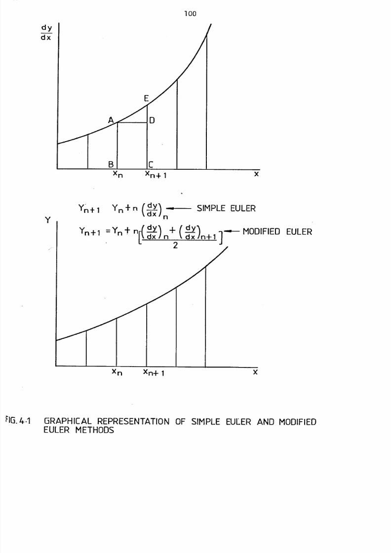
8/6/2019 A. M. Y. Razak Thesis 1984
http://slidepdf.com/reader/full/a-m-y-razak-thesis-1984 114/181
100
dy
dx
B CXn4-1
Yn-+ Yn +n (dy).dx
n
SIMPLEEULER
Yn+l =Yn+ndy
I. *-- MODIFIEDEULER
dx
)
n+
ýd-xy-)n+
1L I-
FIG.-1 GRAPHICAL EPRESENTATIONF SIMPLEEULERAND MODIFIEDEULERMETHODS
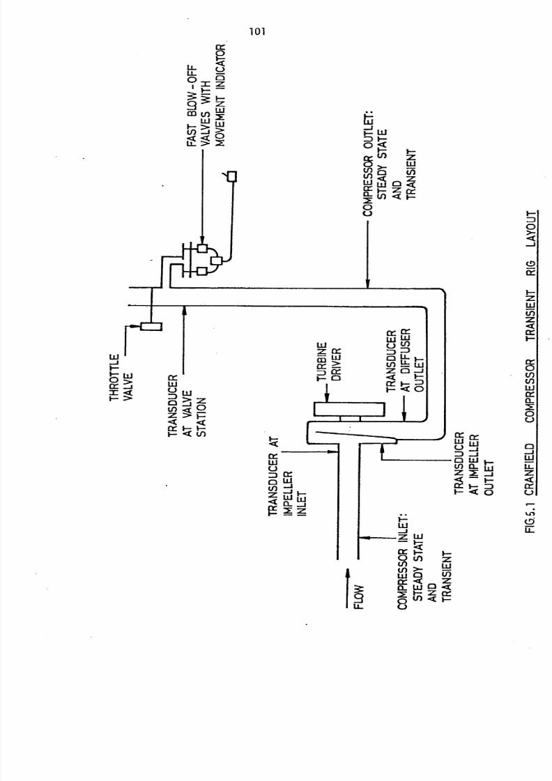
8/6/2019 A. M. Y. Razak Thesis 1984
http://slidepdf.com/reader/full/a-m-y-razak-thesis-1984 115/181
(r_0
LL c)
EimZ
ZU
LU
>, W
L<L
101
LLIz it
ii-aLJ
>
Lýw
0
Ln0(n <WWX tý ccIL < F-M
Lij
LLI fr-o>LLJ
LLI:DC3 >j Z
V) <0z>
cc !ý V-
ý- (n
cr-wu
crLU
Z LU LLj4 Q-Zj
fýMz
LL.
I-
0>-
-J
I-zw
tf)
LLJcr
0u
w crLI LLj
-0LLJ j
LLI
LO CL LLI LLZ 2:
_3z
<<cr- cr-t- <0u
LLJ
-i. 0-Z W
0Z
0wtnwjr- ZCL w0
z Er-
cr cr-
LLI LoMLL
in 4=LLIz0
cr !ýz :Dý- 0
F
0Li
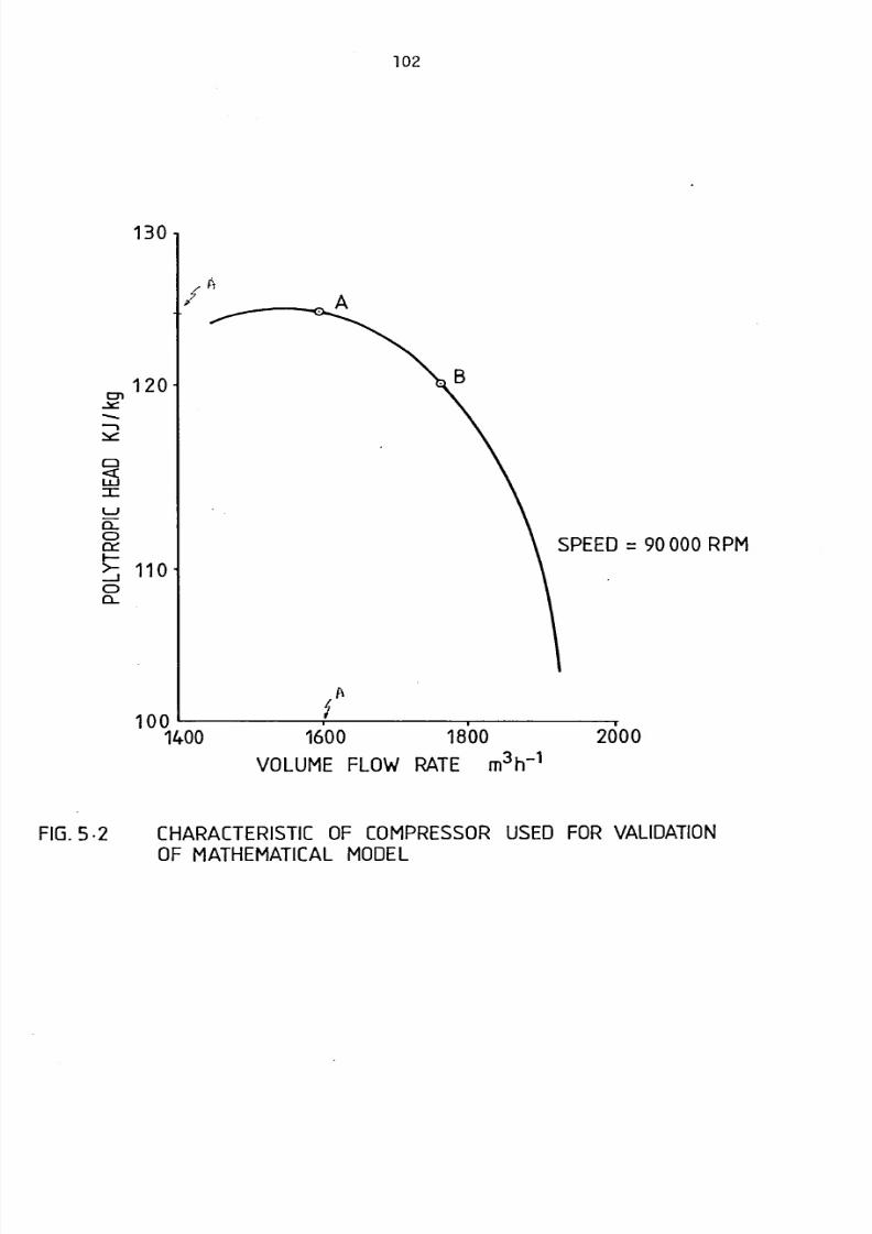
8/6/2019 A. M. Y. Razak Thesis 1984
http://slidepdf.com/reader/full/a-m-y-razak-thesis-1984 116/181
102
1301
cm120
-ICý:
=Li
ä:C:
: 1101.i
C:12-
A I)
I'
Ivv1400 i0o 18,00 2dOO
VOLUMEFLOWRATE M30
FIG.5.2 CHARACTERISTICF COMPRESSORSEDFORVALIDATIONOF MATHEMATICALODEL
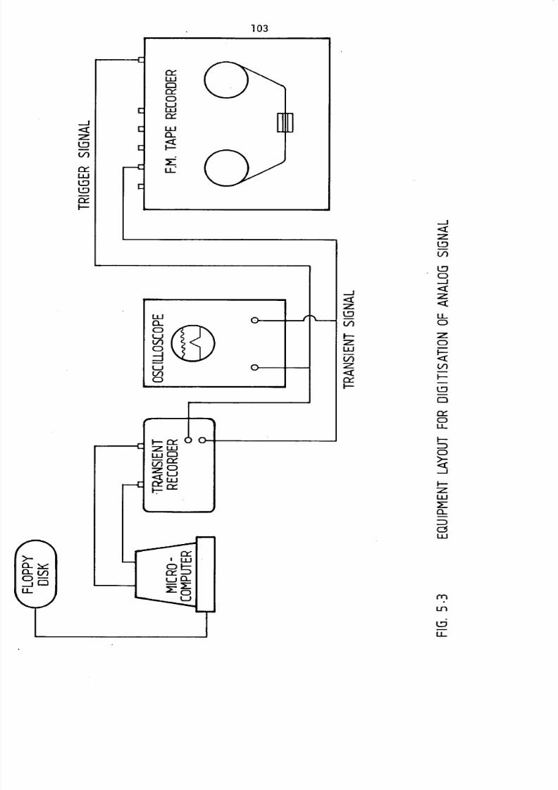
8/6/2019 A. M. Y. Razak Thesis 1984
http://slidepdf.com/reader/full/a-m-y-razak-thesis-1984 117/181
103
LO
cy-LLJLIDLD
-C
:ZLID
(f)
CL
CD
_jC)
LL
r--c
üýLU
r-i12fCDL-i
U-ioý
ui
F--.;
LliCLC)
C)
V)C)
ý- cr::Z LLJ
LLJ
(D
Z LJLUim cr
lý-
Lr
UJ:. J
C:Lj
0 fT%-LIDUl
F--
2-1LU
u)-Z:
(ZCD
LLCD
Z:
C:
F3clýC:LL
CD
:ZLU
Z
rn
Ln
LfjLL
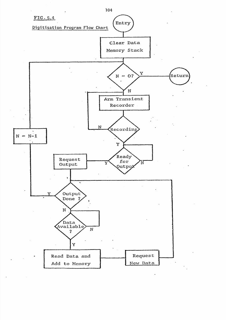
8/6/2019 A. M. Y. Razak Thesis 1984
http://slidepdf.com/reader/full/a-m-y-razak-thesis-1984 118/181
104
FIG-
5.4
Digitisation Program Flow Chart
Clear Data
Memory Stack
Arm Transient
Recorder
N-1
Request
Output
T
I
Read Data and Request
Add to Memory
lqex..
7 Data
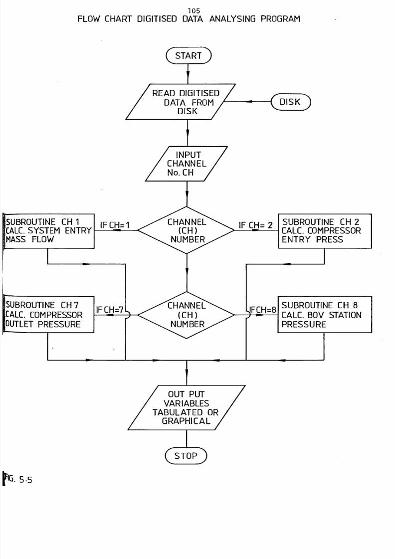
8/6/2019 A. M. Y. Razak Thesis 1984
http://slidepdf.com/reader/full/a-m-y-razak-thesis-1984 119/181
105
FLOWCHARTDIGITISED ATAANALYSINGROGRAM
I
START
/ DC: An nir-.Ticr: nNM
) L) IIjL.
L-DATA
uFROM
)
u.3R
SUBROUTINEH1CALC.YSTEM NTRYMASSFLOW
ýSUBROUTINEH7'ALC.COMPRESSOR[NTLET
PRESSURE
CHANNEL(CH)
NUMBER
CHANNEL(CH)
NUMBER
OUTPUTVARIABLES
TABULATEDORGRAPHICAL
,
SUBROUTINEH2CALC.COMPRESSORENTRY PRESS
SUBROUTINEH 8CALC. OV STATION
PRESSURE
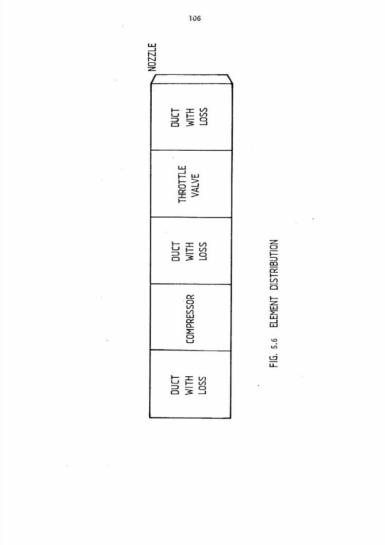
8/6/2019 A. M. Y. Razak Thesis 1984
http://slidepdf.com/reader/full/a-m-y-razak-thesis-1984 120/181
106
LU
NCDZ:
1--_M
L/1Li F- Ln
LLJ
>C: ) --J
<
ulLJ L/1
ZD 59
C:L/1V)
ui
C:Li
v)
C:
c3-.i
2mCD
m
ry-
EAC3
k-Z:
LU-iLLI
U)
U-
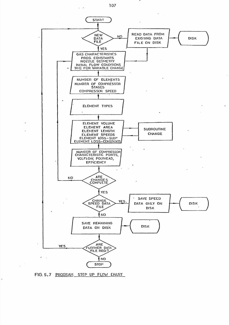
8/6/2019 A. M. Y. Razak Thesis 1984
http://slidepdf.com/reader/full/a-m-y-razak-thesis-1984 121/181
107
GAS CHARACTERISTIC5
PROG. CONSTANTSNOZ2LE GEOMETRY
INITIAL FLOW CONUTIONSTIM. FOR YAR!ABLE CHANGE
NUMBER OF ELEMTNTS
NUMBER OF COMPRESSORSTAGES
COMPRESSOR SPEED
I ELEMENT VOLUME
ELEMENT AREA
ELEMENT LENGTH
I ELEMENT SPEEDSI ELEMENT LOSS-SLOP
I ELEMENTLOSS- CONSTANTS
II NUMBER OF COMPRESSORI CHARACTERISTICPOINTS.I VOLFLOW,POLYHEAD,
EFFICIENCY
READ DATA FROM
EXISIING DATA
FILE ON DISK
NO
SAVE REMAINING
DATA Disk
(:
DI K0.4
I
FIG. 5.7 PROGRA',-', STEP UP FLOW CHART
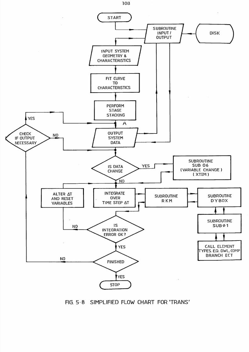
8/6/2019 A. M. Y. Razak Thesis 1984
http://slidepdf.com/reader/full/a-m-y-razak-thesis-1984 122/181
108
I
INPUTSYSTEMGEOMETRY
CHARACTERISTICS
FITCURVETO
CHARACTERISTICS
PERFORMSTAGE
STACKING
CHECKIF OUTPUT
NECESSARY
ALTER AT
AND RESET
VARIABLES
OUTPUTSYSTEM
DATA
IS DATACHANGE
INTEGRATEOVER
TIMESTEPAT
is
INTEGRATION
ERROROK?
FINISHED
SUBROUTINEINPUTOUTPUT
SUBROUTINE
RKM
FIG. -8 SIMPLIFIEDLOWCHART OR'TRANS'
ýSTARTýR
DISK
SUBROUTINESUB06
(VARIABLE HANGE( XTIM)
SUBROUTINE
DYBDX
SUBROUTINESUB01
CALL ELEMENTYPES.EJa.DWL,COMP
BRANCH ECT
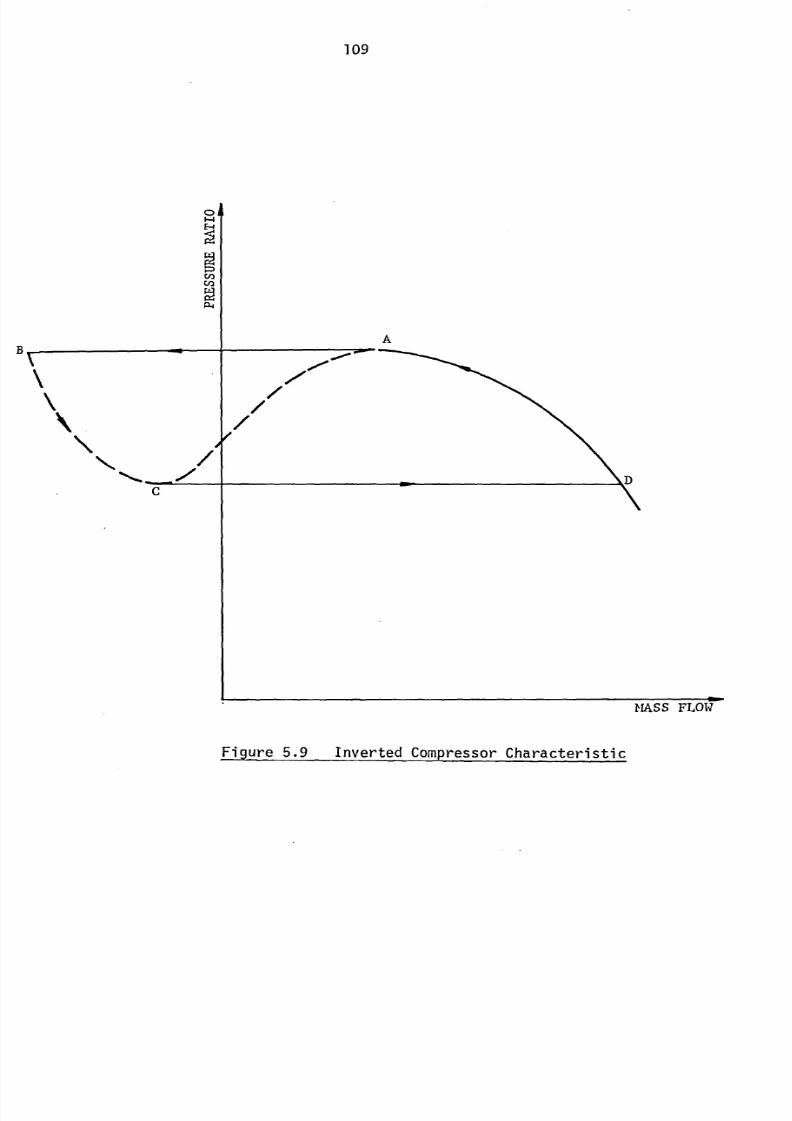
8/6/2019 A. M. Y. Razak Thesis 1984
http://slidepdf.com/reader/full/a-m-y-razak-thesis-1984 123/181
109
B
\
N/C
E-4
V.-/
//
A
MASS FLOW
Figure 5.9 Inverted Compressor Characteristic
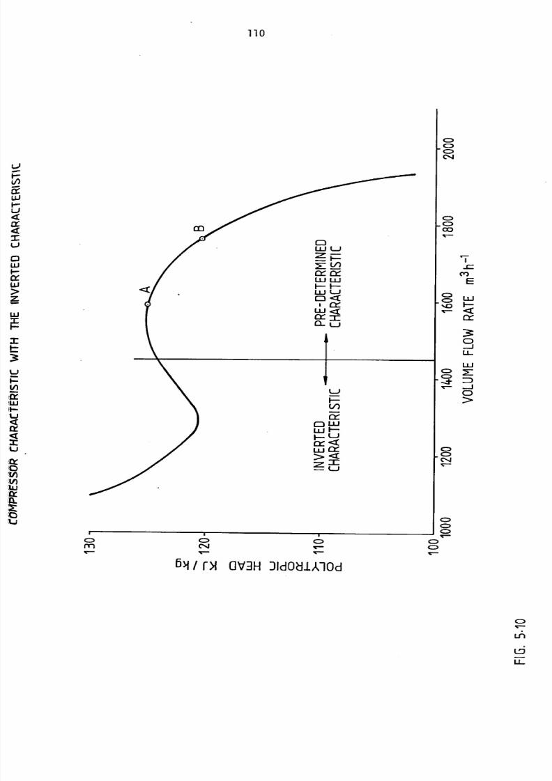
8/6/2019 A. M. Y. Razak Thesis 1984
http://slidepdf.com/reader/full/a-m-y-razak-thesis-1984 124/181
110
u
t17
15L4ty-9c
LU
i-Ofui
Z
w
viIE
Li
VI(V)
I.
tI
-v-
MLLJ L-)
;zpz V)Of IxLLJLUý-- F-LU Ljc: l
LLJ
CX0.-LJ
V)E
C: LuLLJF-ý-- LJcc: <
LU
rL-)
6Mf >1 OV3HIdOdl)Md
C>
C)C>Co
ýr-
C)
C>CDIt
C14V-
C=)
CY)
E
LLJ
C)-iLL-
LLJ
CD
Ir-
LALO
E
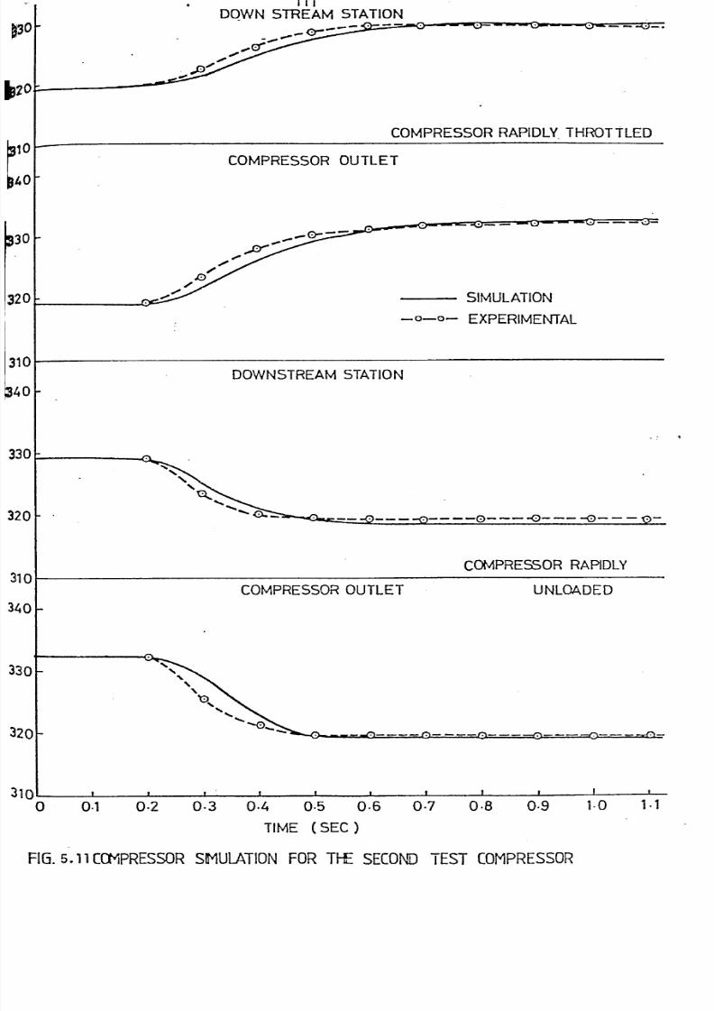
8/6/2019 A. M. Y. Razak Thesis 1984
http://slidepdf.com/reader/full/a-m-y-razak-thesis-1984 125/181
IIIDOWN STREAM STATION
030
b7o
40
30
320
310
40
330
320
310
340
330
320
31()
COMPRESSOR OUTLET
COMPRESSOR RAPIDLY.THROTTLED
- SIMULATION
-0-0- EXPERIMENTAL
DOWNSTREAMSTATION
COMPRESSORUTLET
COMPRESSORRAPiDLY
UNLOADED
0 0-1 0.2 0.3 0.4 0.5 0.6 0-7 0.8 0.9 1.0
TIME (SEC )
FIG.5.11COMPRESSORIMULATIONORTHESECONDESTCOMPRESSOR
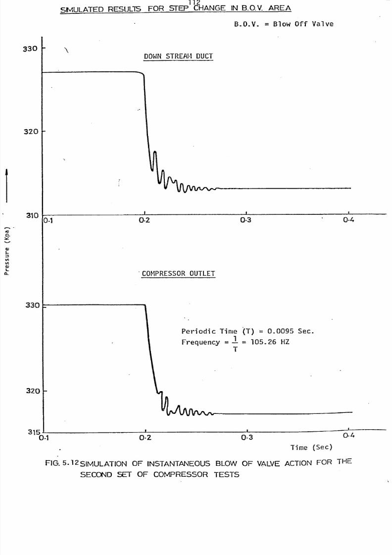
8/6/2019 A. M. Y. Razak Thesis 1984
http://slidepdf.com/reader/full/a-m-y-razak-thesis-1984 126/181
112
SMULATED RESULIS FOR STEP CHANGE IN B.O.V. AREA
B-O.V. = Blow Olf Valve
330
320
DOWN TREAM UCT
I
310
330
0.1 0-2 0-3
. COMPRESSORUTLET
Periodic Time (T) = 0.0095 Sec.
Frequency =-l = 105.26 HZT
320
0.4
3151 tof-1 0-2 -3
0-4
Time (Sec)
FIG.5.12SIMULATIONOF INSTANTANEOUSLOW OF V,LVE ACTIONFOR THE
SECONDSET OF COMPRESSOR ESTS
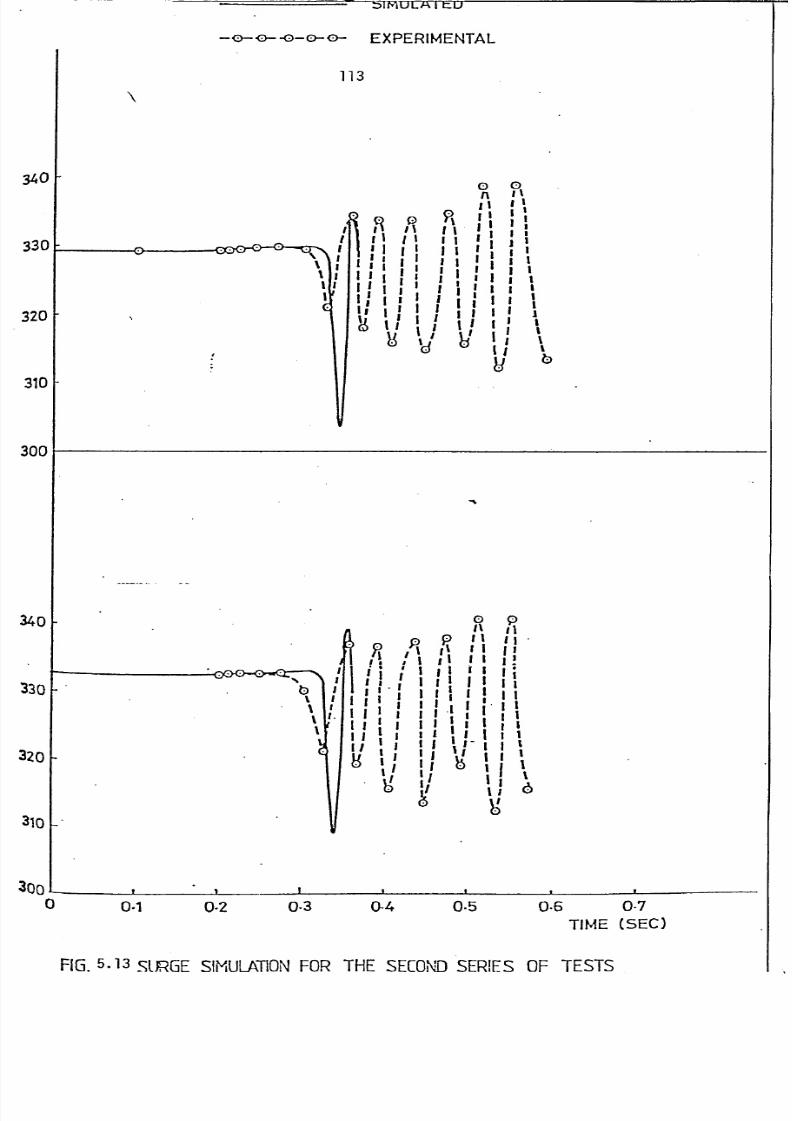
8/6/2019 A. M. Y. Razak Thesis 1984
http://slidepdf.com/reader/full/a-m-y-razak-thesis-1984 127/181
---5TMULA I LU
EXPERIMENTAL
113
340
330
320
310
300
340
330
320
31()
3000
I- ,
0011 ig%
R: ' It tI 11 It Ii
I II I II I ii. 11111IIS I,
II ji IIIi IiIII
11 IIII ii
I
SI
opi 11
5 Ip
p
it it.% gt ii 1I, gt tIi!j' IIij;
".. ii Iib iiji" fI ItI
jI .111It 1II III
II'I£II ii
I, II tI-i I'I'lIi I
Ilt
ti a
I---
IfII---. -I
0-1 0-2 0-3 0-4 0.5 0-6 0-7
TIME (SEC)
FIG.5.13 - ' - THE TESTS
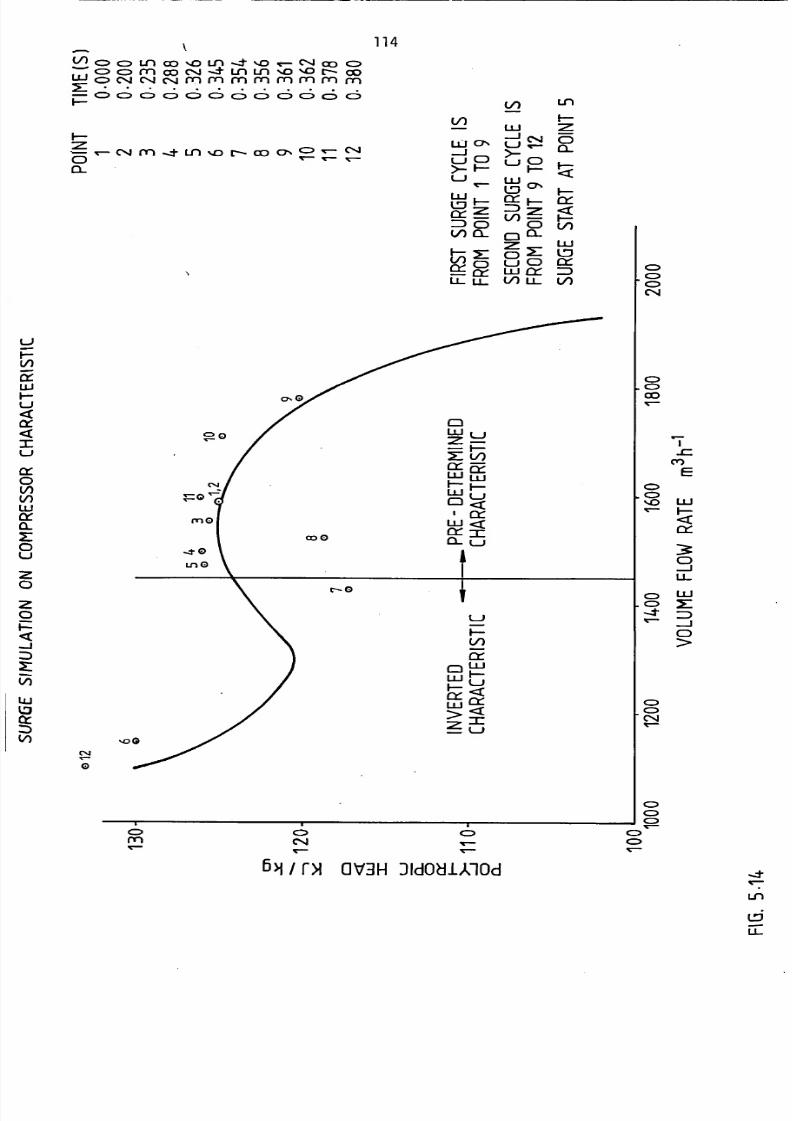
8/6/2019 A. M. Y. Razak Thesis 1984
http://slidepdf.com/reader/full/a-m-y-razak-thesis-1984 128/181
k
(A c> c) Ln cc)%o r) -t %D v-- C%4m c>c-! i e---, rn ei; -%ni -+ i ri t ri -, i %n F-- ;;%
M riý Fri iý-i ýn-M ýn
C=)666C: ) C) c:: C>C) CD
F--:Z,
c-4m -d-Lri %o , co (7,cD- c*4CD12-
co0
LU
CY :zZ: C:V) CL
I-- yV)Cy CD
OfU-
Q0
C4
-t 0
Ln 0
r- 0
V)
L. J CD
Li
MLU L-JM FZ-K V)cr- ? YLLJ LL.JF- ý-LJ
LjM<
I Q::Lu <Qr- -T-Cl. L-)
V)E
m LU
Lu ý7- %-j
r-ini:
<
Lij
Z Li
C14
,.Do
C) C>rn C44V- T- v-
rA OV3H31dOdUlOd
114
L/)
LLJ
-i (NLJ
t-.J CDF-
LL.LO
=: ) 7:V)
C)C:
CDLj CDLLJOfV) LL
Lr)
C)
LLJ
4=>C>C>CN
C)CDaoV-
C)
I C)C>-tvl--
C)C:)CN
C>CD
C>C)
V-
V-
cn
E
LLJ
F-
C)I
U-
LLJ
CD
-t'17Ln
6
LL
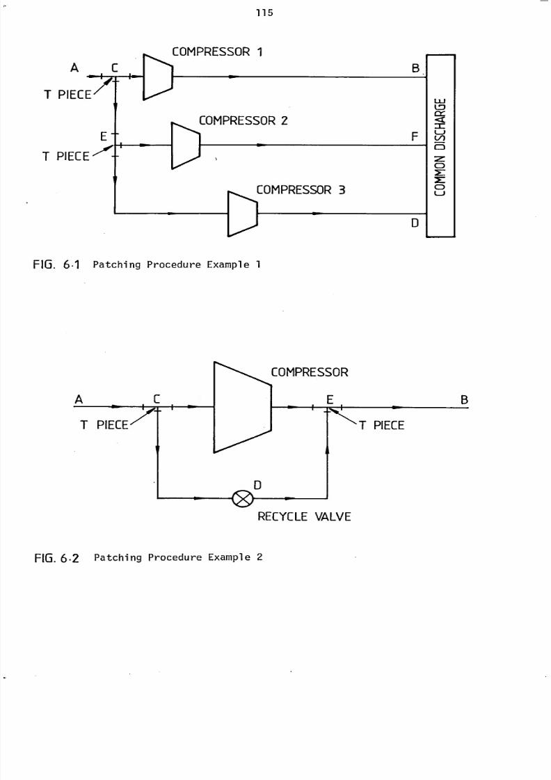
8/6/2019 A. M. Y. Razak Thesis 1984
http://slidepdf.com/reader/full/a-m-y-razak-thesis-1984 129/181
115
A
T PIECE
T PIECE-'
I
r. -ýCOMPRESSOR
Ll--ý
COMPRESSORrll<
COMPRESSOR
40ý
FIG. 6.1 Patching Procedure ExampleI
RECYCLEALVE
LLJ
Lo
=Li
D
D
0LI
FIG.6.2 Patching Procedure Example 2
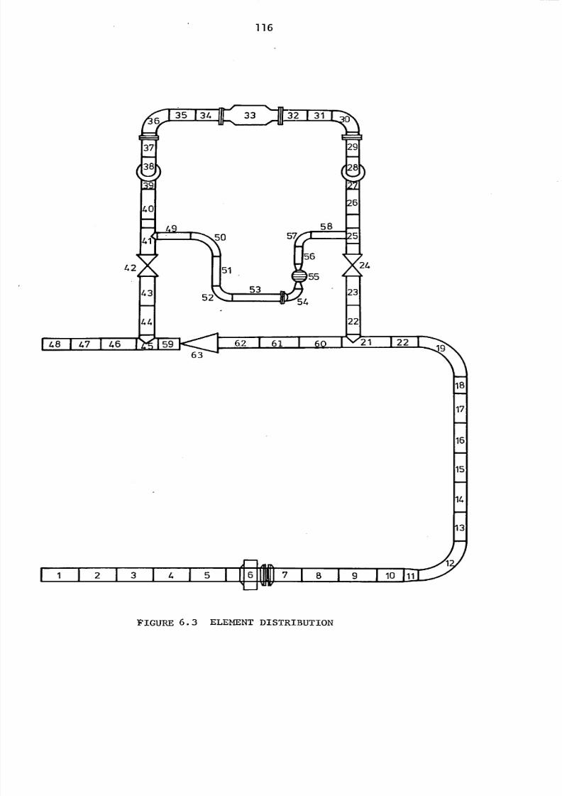
8/6/2019 A. M. Y. Razak Thesis 1984
http://slidepdf.com/reader/full/a-m-y-razak-thesis-1984 130/181
116
FIGURE 6.3 ELEMENT DISTRIBUTION
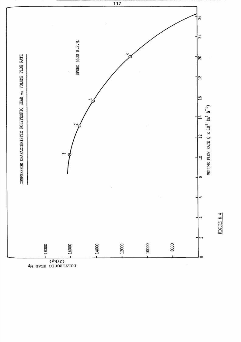
8/6/2019 A. M. Y. Razak Thesis 1984
http://slidepdf.com/reader/full/a-m-y-razak-thesis-1984 131/181
117
0Lri
%Z
tz
ul
E
c
E
H
-:TC14
cqcq
0C14
00
-4
-4
.4T
C14
-4
0-4
OD
1.0
--zr
I-.
C"
E
m0
E-4
CD
0
1:4
Co %0 -zr cq
(SVOdM C[V21H iaoxirioa
C)
0 03
N
0
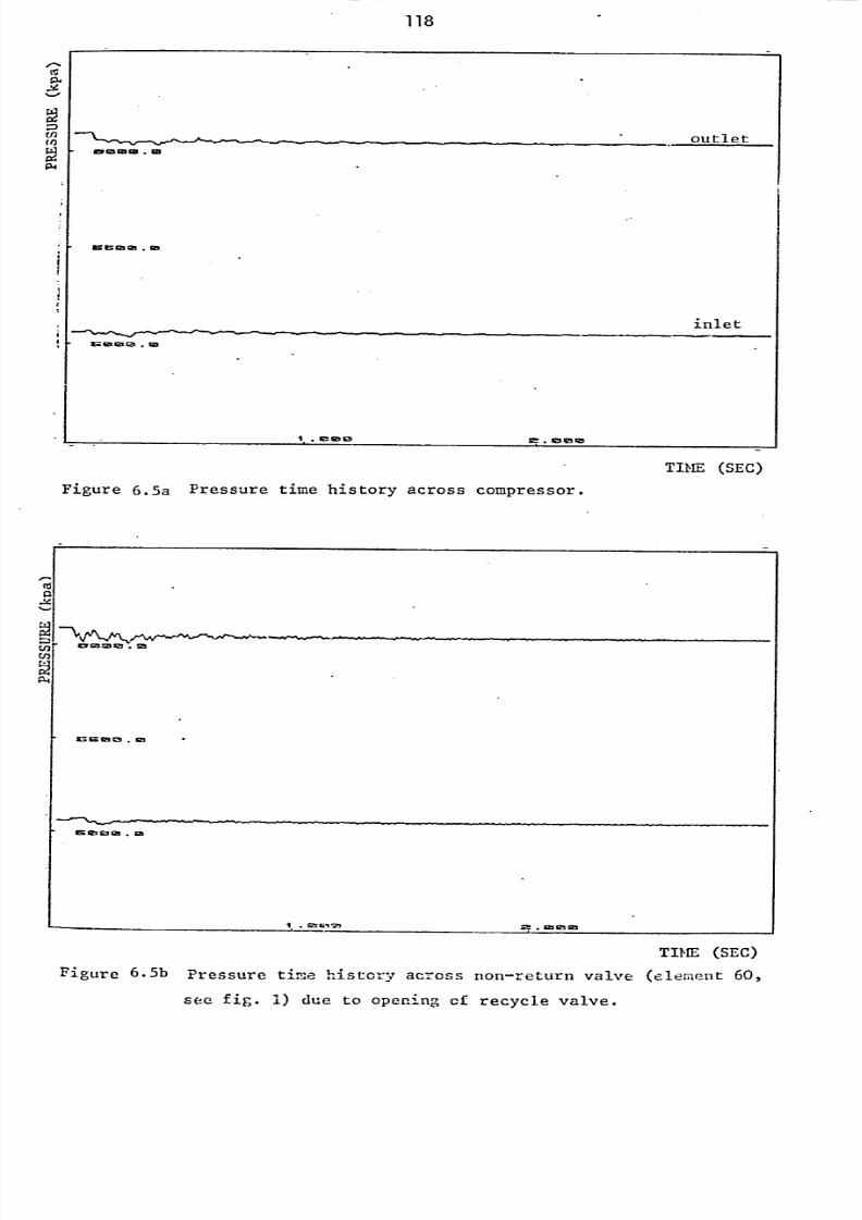
8/6/2019 A. M. Y. Razak Thesis 1984
http://slidepdf.com/reader/full/a-m-y-razak-thesis-1984 132/181
118
I-,.
54
t/2C/2
Me G503 SO.m
wr. sa 122
.in
NUel23C2N
.la
. IENGD43 a. 0010
Figure 6.5a Pressure time history across compressor.
Wcl
p. 4
ý. 1211.1 VM z7-
123 929 cm
outlet
inlet
TIME (SEC)
TIME (SEC)
Figure 6.5b Pressure time history across non-return valve (ele, -, ,Cnt 60,
see fig. 1) due to opening cf recycle valve.
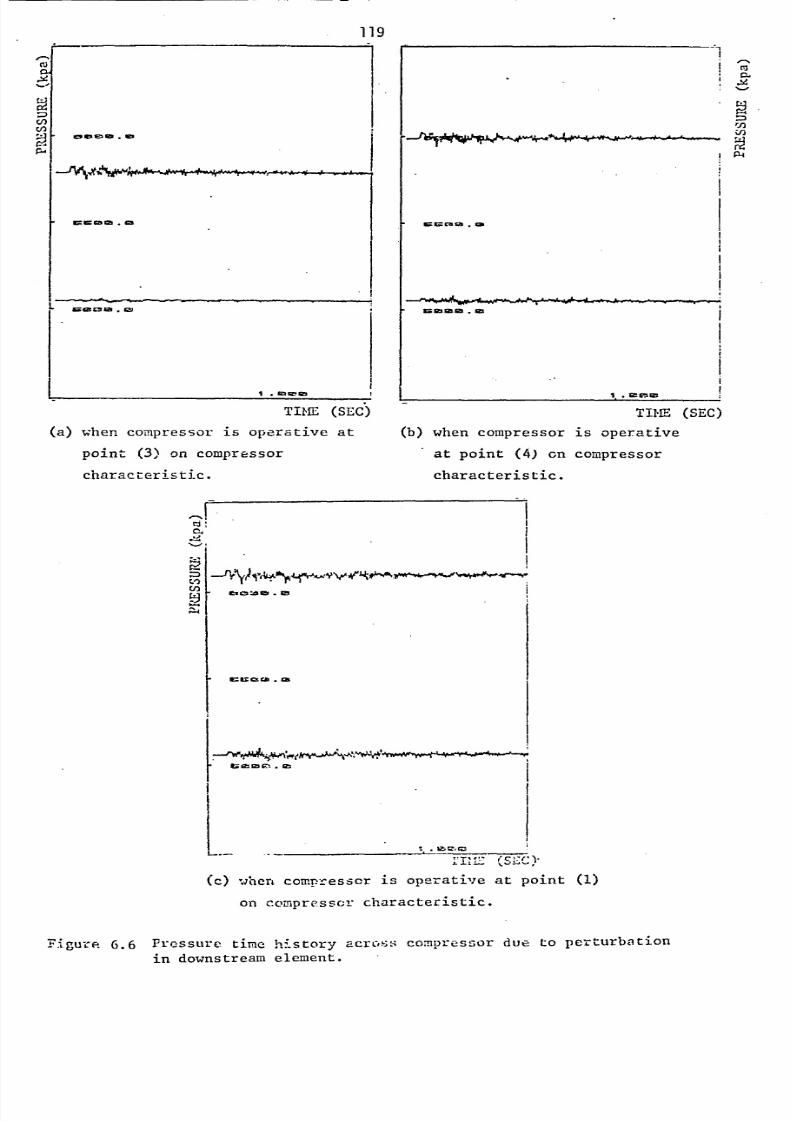
8/6/2019 A. M. Y. Razak Thesis 1984
http://slidepdf.com/reader/full/a-m-y-razak-thesis-1984 133/181
119
'-a
C,Cl)
esec"ll . 10
- . --. -J--
I
u1r. Kaim . da
=9293ift e2
i. Am V Go
TIME (SEC)I.
sm ol as
TIME (SEC)
(a) when couipressor is operative at (b) when compressor is operative
point (3) an compressor at point (4) on compressor
characteristic. characteristic.
I!rj :C4
:0V)Cl)
L4 cs za I&.
125
ntzacb. cat
U as
I
1_
r== ra a. a
1--vi la in. la
.Ib tzýr_-
Ia: (sEC)(c) when compressor is operative at point (1)
on compresscr characteristic.
F-*, u-cr-. 6.6 Frossure time history acroý-,! compressor due to perturbation
in downstream element.
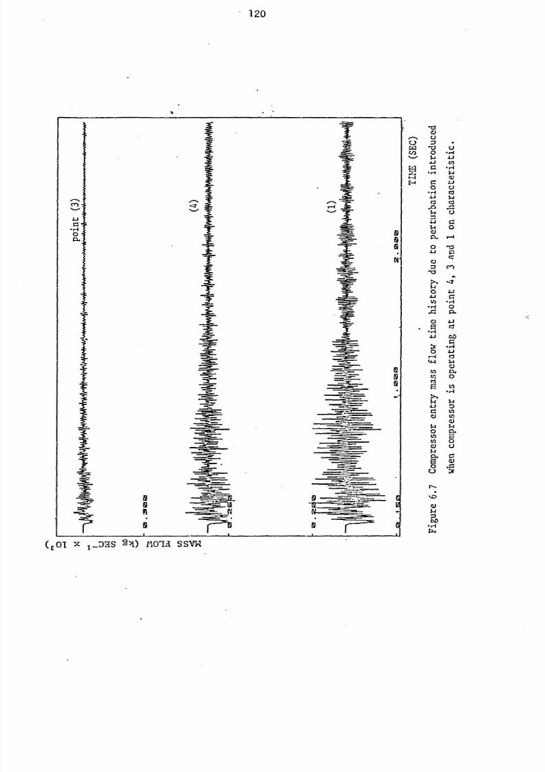
8/6/2019 A. M. Y. Razak Thesis 1984
http://slidepdf.com/reader/full/a-m-y-razak-thesis-1984 134/181
. 120
C/3
r:0
. rq4-1
04
0
41
,a
-r441
It
0
-444
to
41
t.,
W
&4
0
W
ti)
(1)$4
0
ri
bO
6r4
4J
41U0$1
u
r.0
1-4
10P.C,,
C?
I%zr
0
P.
4-1Cd
410$4
0
to
0
(coi x 1-D2S4) Molil SSVN
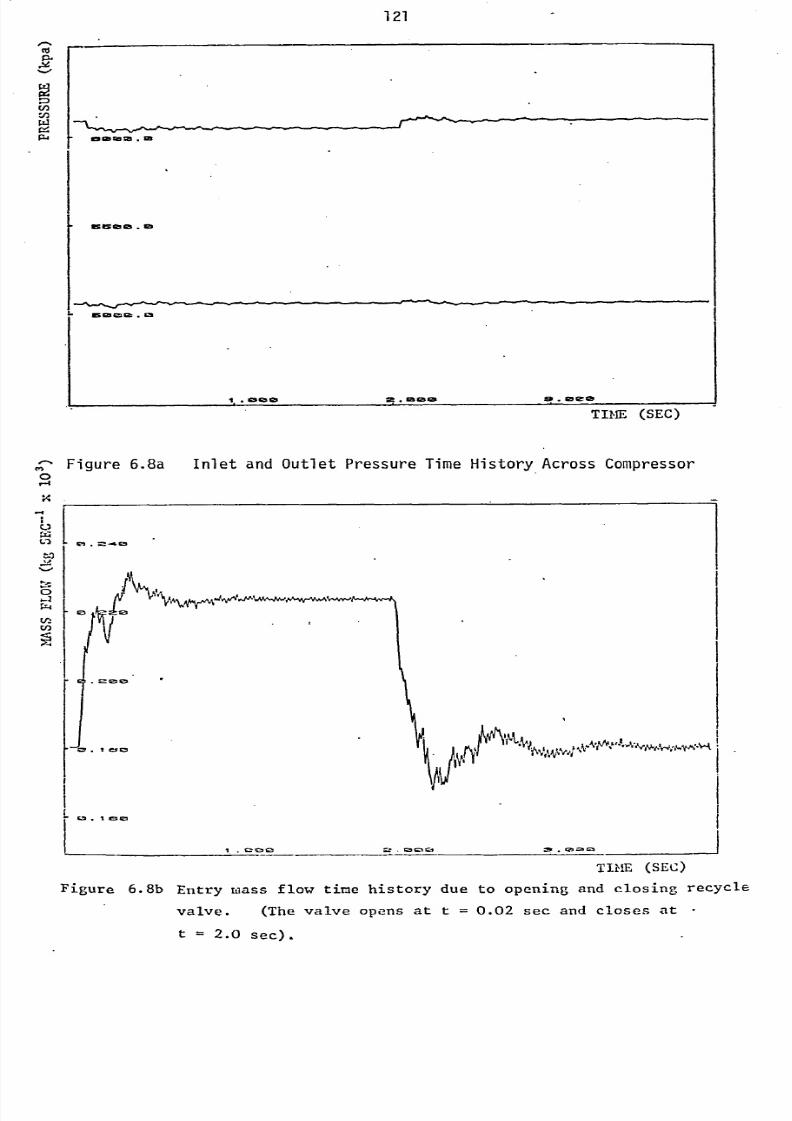
8/6/2019 A. M. Y. Razak Thesis 1984
http://slidepdf.com/reader/full/a-m-y-razak-thesis-1984 135/181
121
e-Ito92.
En
C4r4
9smsomm
Isislao. la
2512209bsm
1. . 10010 ze . laga4iN 0.000
TIME (SEC)
Figure 6.8a Inlet and Outlet Pressure Time History Across Compressor
0-4
1,C-.
Lý0
V-1
NAA
.
r &5.1 950
I.Ll C. 0 r_-
.so ala ýN . (? ?ca
TII, M, (SEC)
Figure 6.8b Entry mass flow time history due to opening and closing recycle
valve. (The valve opens at t=0.02 sec and closes at -
t=2.0 sec).
". ;aýrD
I y,V,,.
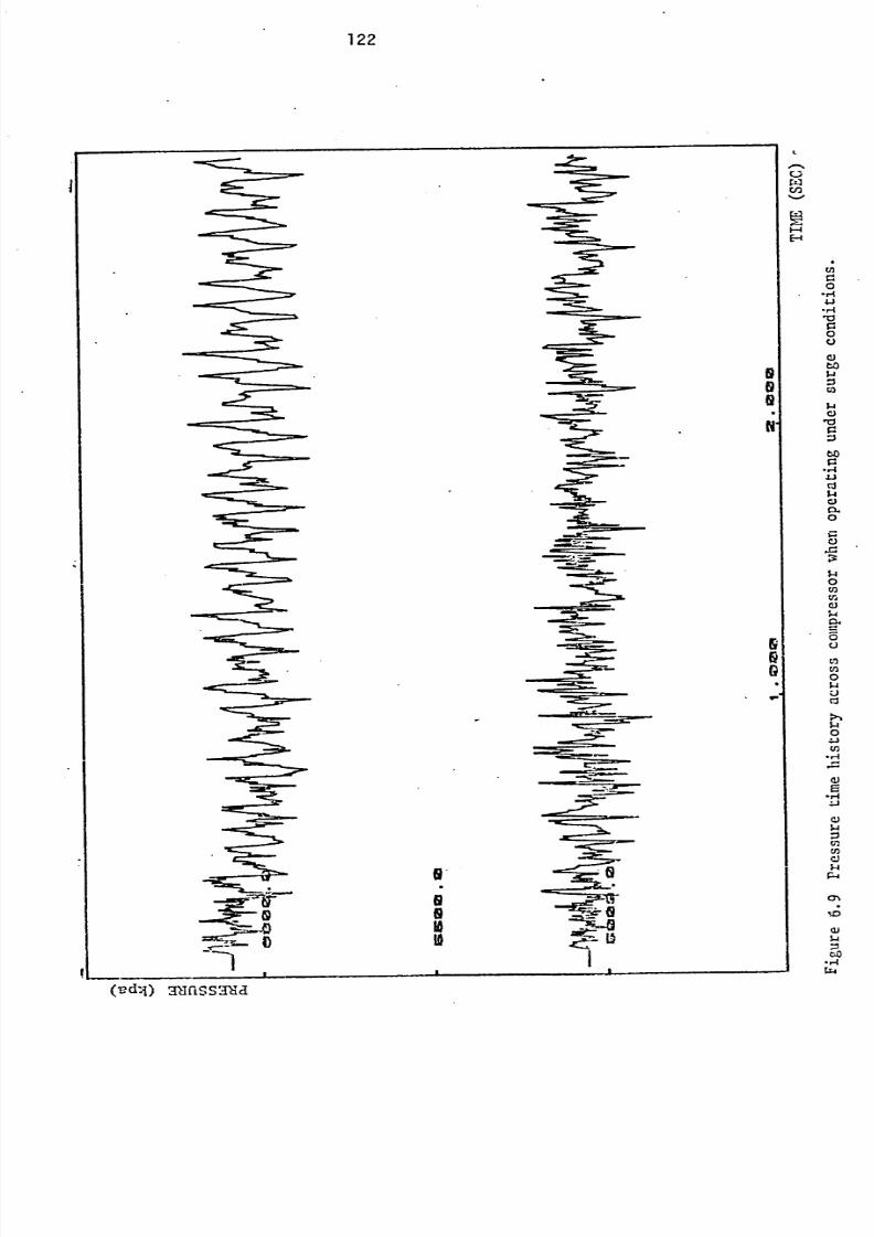
8/6/2019 A. M. Y. Razak Thesis 1984
http://slidepdf.com/reader/full/a-m-y-razak-thesis-1984 136/181
I
3; 7
-a-
(-ed: ) gurt-, sgul
M.
122
aN
w
-- --e_--
i22ý
I!
z1
ý2E-4
N
N
&
I-
0
,0
LG
tricl);4
C)
0cn0
0Z-3rA
w
., irJ4
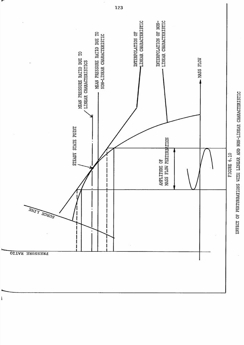
8/6/2019 A. M. Y. Razak Thesis 1984
http://slidepdf.com/reader/full/a-m-y-razak-thesis-1984 137/181
123
6ý
-iýz6l
Oliva missaua
0E-1U
HW E-Azo coP F-4
r4ý-q E-4
00E-i
En
0 E-4 En1-4 En EnE--l " wW
P4L4
z
A4 P4
.cZ
ý"1'
N
I
!ý"C23
F-IE-4 0 E-4U) z U)F-I H
rM4 P4 rX4 P4
0w0W
E-4 E-4z0z0
00
0
wwwwE-4Zz
F-4 F-I
ý-l 00
rZ4 W0 PLI
w
E-4 FM4H
0-1 ri)
I
I
ý3:0ý4
I
0
P4
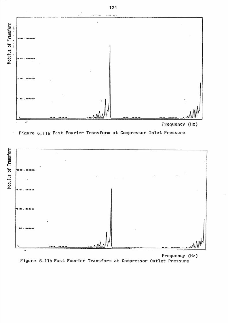
8/6/2019 A. M. Y. Razak Thesis 1984
http://slidepdf.com/reader/full/a-m-y-razak-thesis-1984 138/181
124
E-0ý
h- -ta . %a%aM
rl U. 0.35!,
t1l G5 . IMMO
I
.I
t- S. CMS3 C21
Frequency (Hz)
Figure 6.11a Fast Fourier Transform at Compressor Inlet Pressure
E0-
r2m 'a . or.! %el
I W. loolla
rl la . lagala
I
I
r 15 . onsaim
I_________________________________ __________________
Frequency (Hz)
Figure 6.11b Fast Fourier Transform at Compressor Outlet Pressure
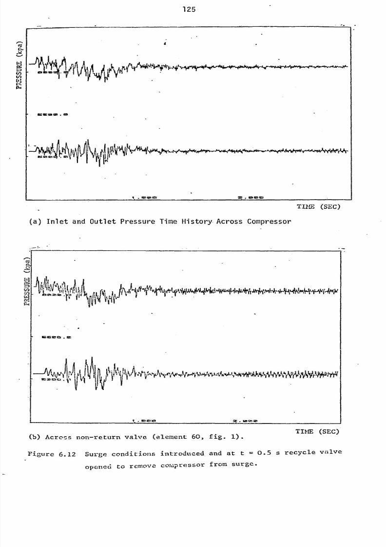
8/6/2019 A. M. Y. Razak Thesis 1984
http://slidepdf.com/reader/full/a-m-y-razak-thesis-1984 139/181
125
I
I- wisimal921
I tolms 9!1 =. ID OD121
TIME (SEC)
(a) Inletand
Outlet Pressure Time History-Across Compressor
r
U)
p4
wsleft. m
rill,
ý,I--mitm'Vill
I I. so al ta ts--Mrl-mm
(b) Across non-return valve (element 60, fig. 1).TIME (SEC)
Figure 6.12 Surge conditions introduced and at t=0.5 s recycle valve
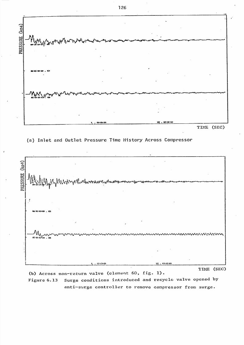
8/6/2019 A. M. Y. Razak Thesis 1984
http://slidepdf.com/reader/full/a-m-y-razak-thesis-1984 140/181
126
Cd0
%-W
M 115
yl ý21d,
^A
4m r. ib w. 10
""
(a) Inletand
Outlet Pressure Time History Across Compressor
CL
cJU)
TLDiE (SEC)
1-. r_- es 21.
cm
-/ V WL%ýc3C--ea
.im
1ý.= ---3 Zý. la cnQ5
(b) Across non-return valve (element 60, fig. 1).MIE (SEC)
Figure 6.13 Surge conditions introduced and recycle valve opened by
anti-surge controller to remove compressor from surge.
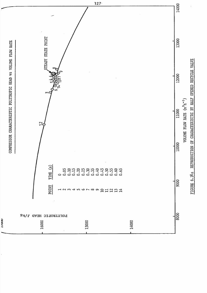
8/6/2019 A. M. Y. Razak Thesis 1984
http://slidepdf.com/reader/full/a-m-y-razak-thesis-1984 141/181
127-
SýIlf (IVHH DICIOUMOCI
0CD0%M, -4
I
0
Ln -17-4 1-4
II
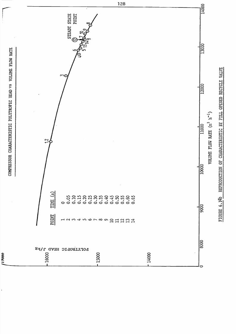
8/6/2019 A. M. Y. Razak Thesis 1984
http://slidepdf.com/reader/full/a-m-y-razak-thesis-1984 142/181
1218 I'll,
21/f (IVHH DIJOUIXIOcI
00 CD000000
Ln -,r-4 r-A
5
0
C)
C14r-4
000
0000
000ON
00000
E-49
:3:0F-I
-0
P4
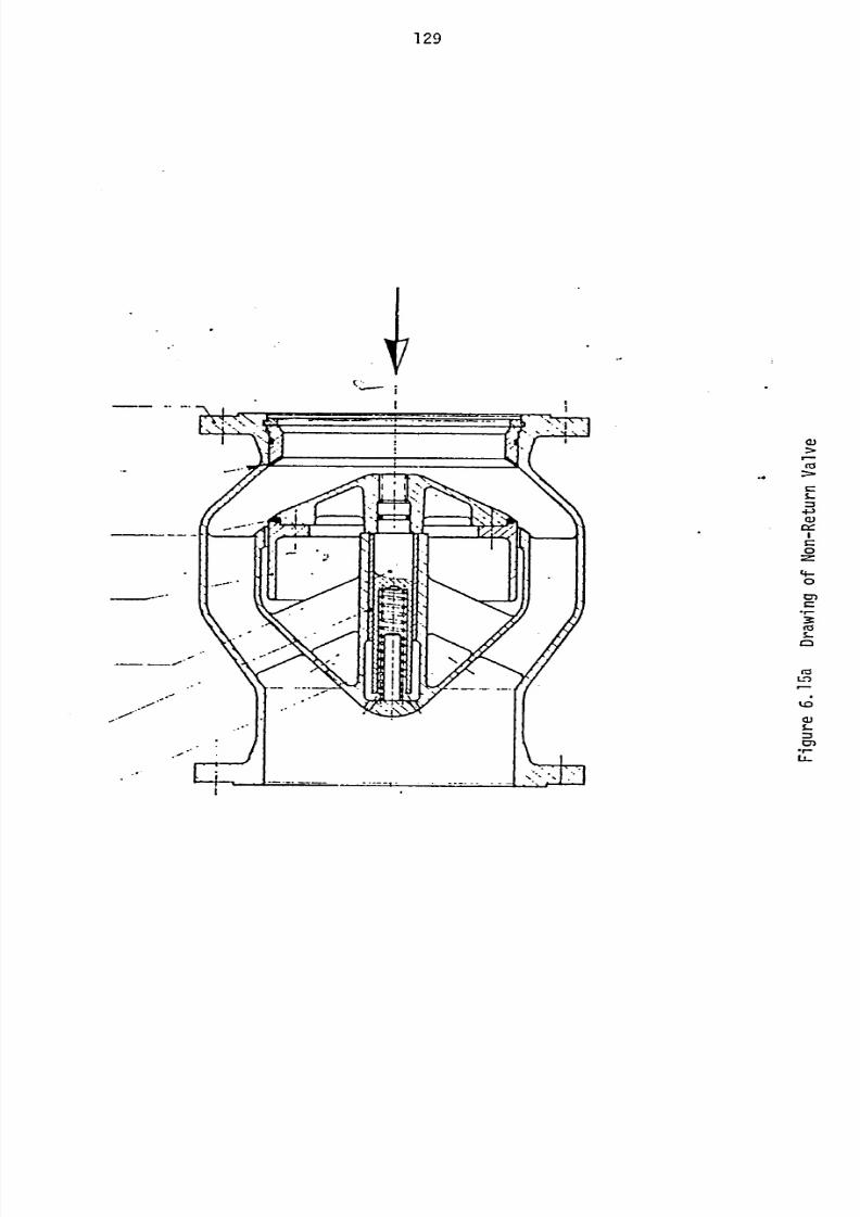
8/6/2019 A. M. Y. Razak Thesis 1984
http://slidepdf.com/reader/full/a-m-y-razak-thesis-1984 143/181
129
Cj
(cs
4Ja)
0
4-0
cn
in
m)
0). r.LL-
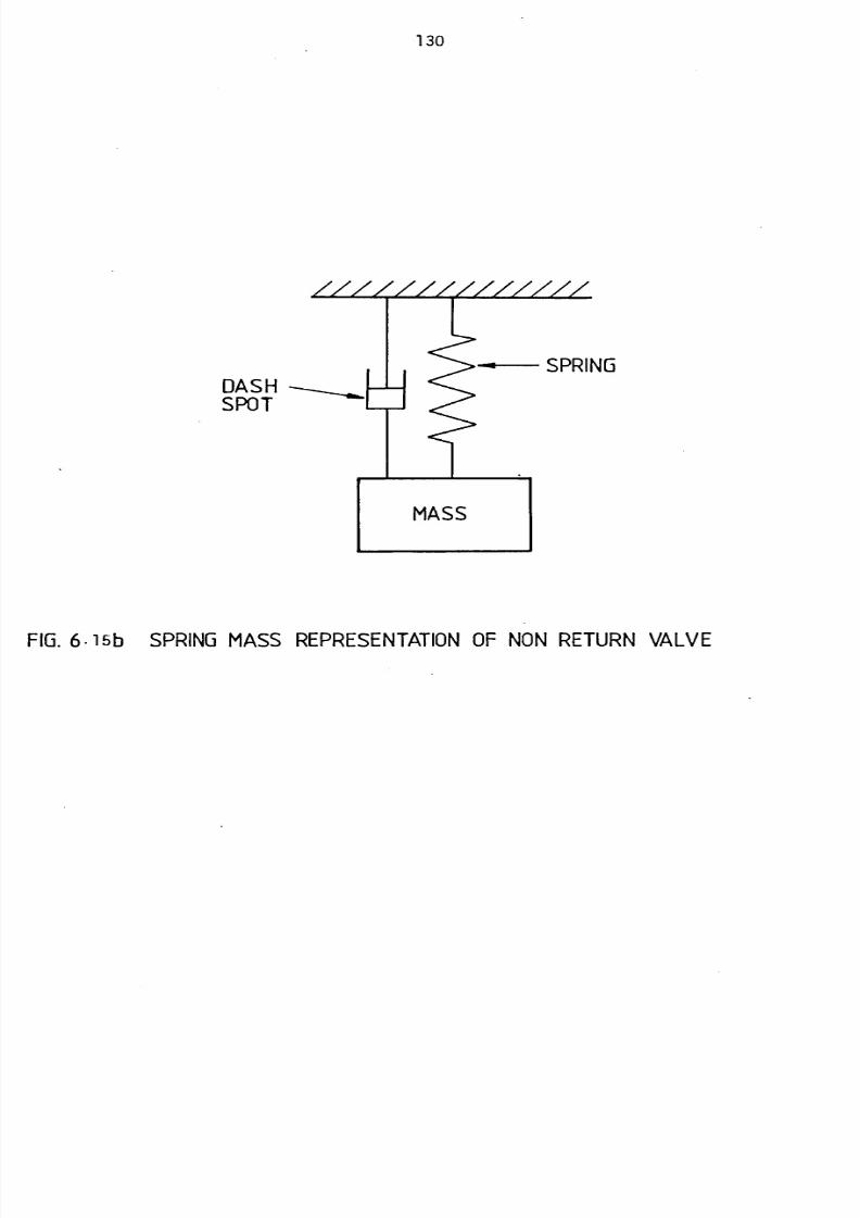
8/6/2019 A. M. Y. Razak Thesis 1984
http://slidepdf.com/reader/full/a-m-y-razak-thesis-1984 144/181
130
DASH
SPOT
FIG.6-15b SPRING ASS REPRESENTATIONF NONRETURN ALVE
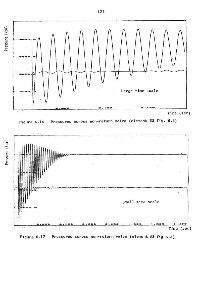
8/6/2019 A. M. Y. Razak Thesis 1984
http://slidepdf.com/reader/full/a-m-y-razak-thesis-1984 145/181
131
10saisla 12? .I
sis
,! - lww
Time (sec)
Figure 6.16 Pressures across non-return valve (element 63 fig. 6.3)
1.1ý0ý
40
Ip
I
if
p
PPVI-
If
Small time scale10. lib
I
q. ýIMG3 ý? . .4cale Qý. 45010 !R. almo 1.
. 130GD 1..
ý00 1... 4010
Time (sec)
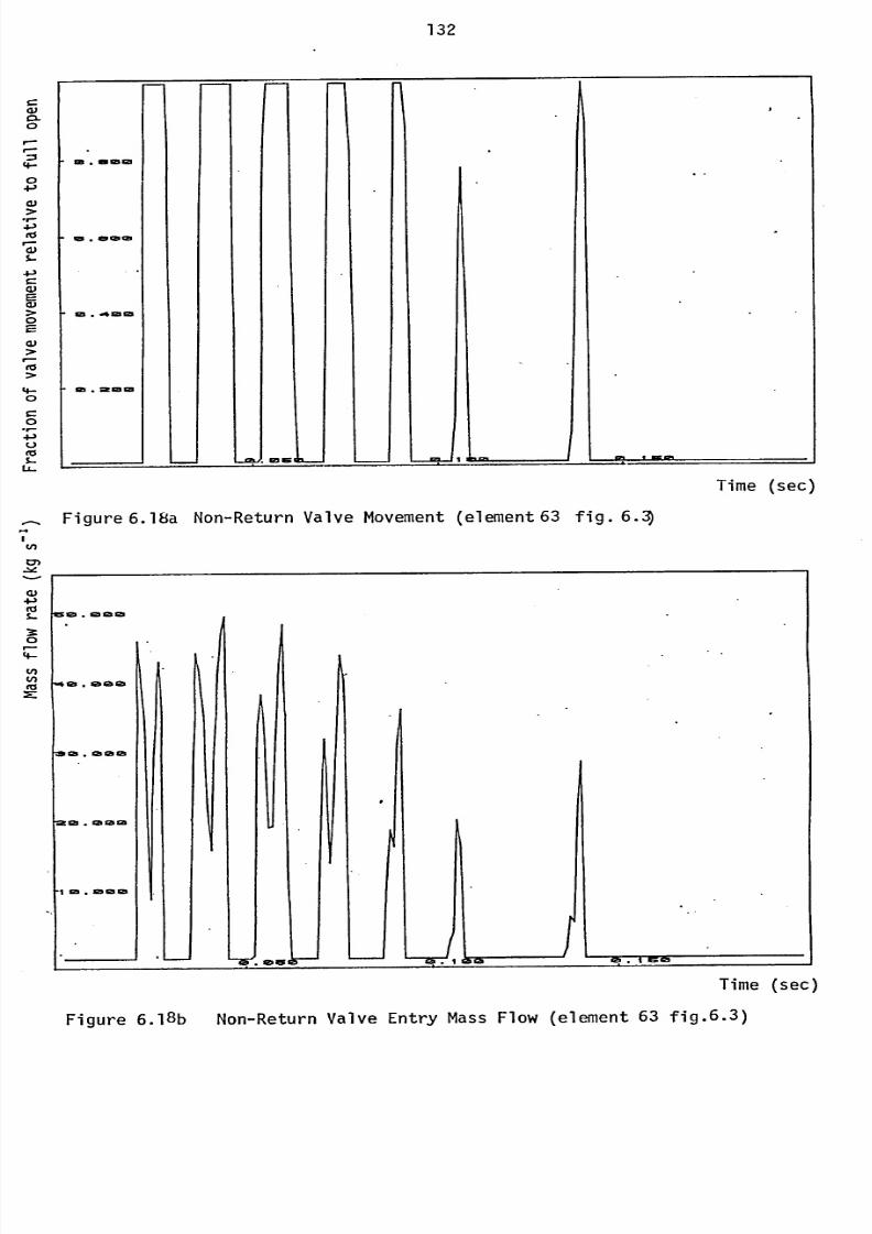
8/6/2019 A. M. Y. Razak Thesis 1984
http://slidepdf.com/reader/full/a-m-y-razak-thesis-1984 146/181
132
4-
04-3
4-)
d)
4-3u
LL-
=. amia
in .43 da cas
t- Im . .4 al a
921Z& In cm
L-jZL/
65S L--JZL-i lbI
J=
Time (sec)
Figure 6.18a Non-Return Valve Movement (element 63 fig. 6-ý
4,
S.
a:0
I-
4-
Z:
Time (sec)
63 6.3)
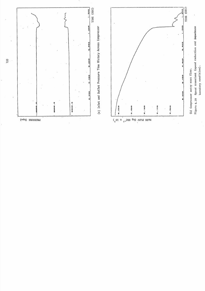
8/6/2019 A. M. Y. Razak Thesis 1984
http://slidepdf.com/reader/full/a-m-y-razak-thesis-1984 147/181
aa
I-S
HE-4
1212
0
ei
S-o(1)
0C-) I
LA
(n0S-
4-3
C)
4-)Q)
UN
44
1-4H
N
C
C
N
N
CN
4-1
4.1
LO
Mci
F-.
Ici
r.ri
"Z;Q;3-4
, Tici(L)
N441
c6)c2.
tn
01%
0, 4
4-J
10
0
.13
(x!dA) n[ISSna (col
x-oas
2ý0 moria svw
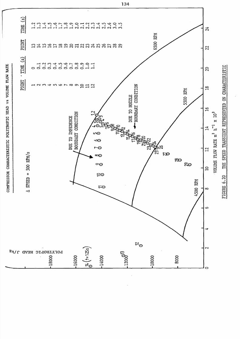
8/6/2019 A. M. Y. Razak Thesis 1984
http://slidepdf.com/reader/full/a-m-y-razak-thesis-1984 148/181
134
e-%
E-A
E-4z
ý-A0Pi
F-IE-f
P-4
P4
22i/f GVHH DICIO'dlxIocl
CD0OD
LnCý4
-0000
r14
(nT--
cli-0
0 OD
-Zrc4
C-4C14
0C'4
00-4
%D-4
C*0
,4
I-.
-:1-I
en
E!WE-4
01-4rZ4
00
%D
, T
(. J
0
0CNI
1180I-I
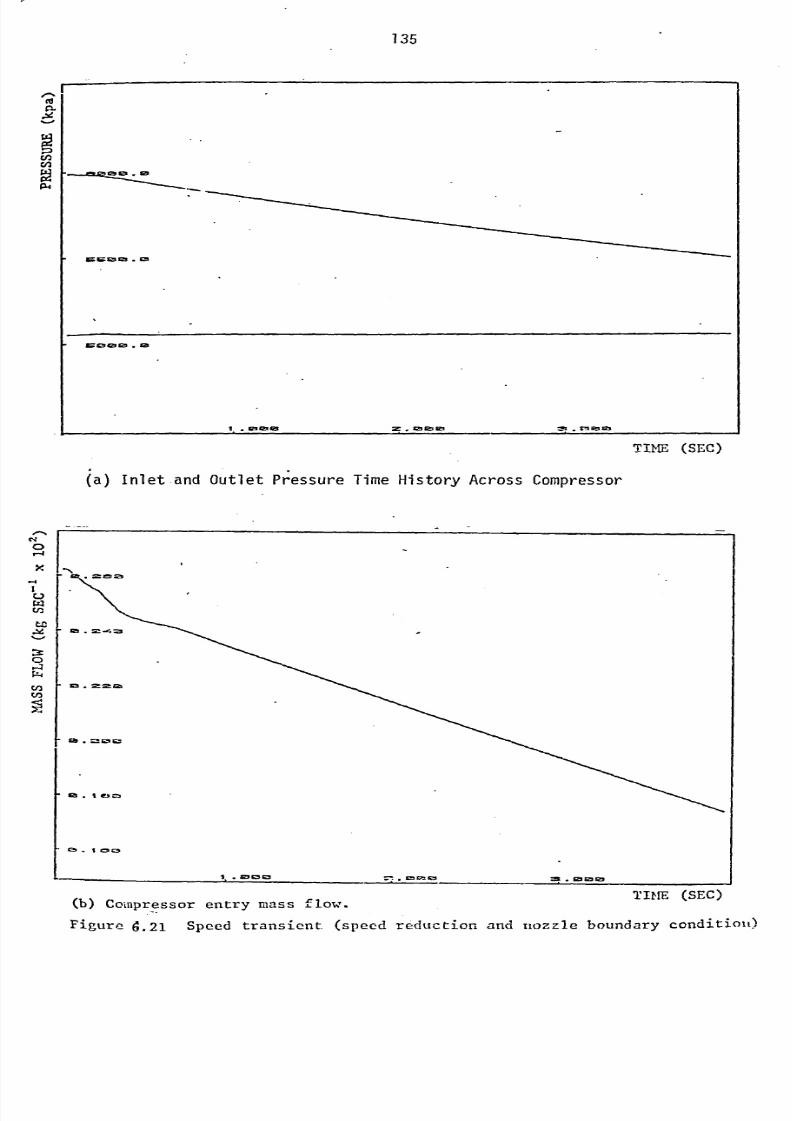
8/6/2019 A. M. Y. Razak Thesis 1984
http://slidepdf.com/reader/full/a-m-y-razak-thesis-1984 149/181
135
I-'
p4
TIME (SEC)
0
-1
C-,
CJj
.2
0
ýa) Inlet and Outlet Pressure Time History Across Compressor
12ý.1 45 C3
I. sn r5 0
(b) Compressor entry mass flow.
r7 . smi"" =. sm so 122
TIME (SEC)
'Figure 6.21 Speed transient (speed reduction and boundary condition)
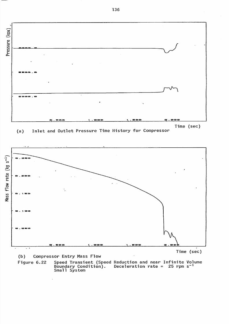
8/6/2019 A. M. Y. Razak Thesis 1984
http://slidepdf.com/reader/full/a-m-y-razak-thesis-1984 150/181
136
CL
amCh C29
.Gh
ocalmeD . ]a
Cý. is Inca 1. . la la la 1. . ms ssa Sý. 1000
(a) Inlet and Outlet Pressure Time History for Compressor
Time (sec)
I
0)
Itsz
Time (sec)
(b) C.mpressor Entry Mass Flow
Figure 6.22 Speed Transient (Speed Reduction and near Infinite Volume
Boundary Condition). Deceleration rate = 25 rpm s-1
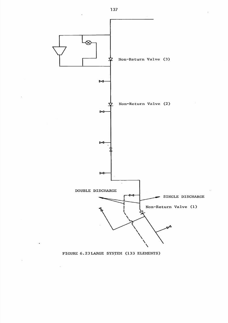
8/6/2019 A. M. Y. Razak Thesis 1984
http://slidepdf.com/reader/full/a-m-y-razak-thesis-1984 151/181
137
to_,u
Non-Return Valve (3)
Non-Return Valve (2)
"---i
FIGURE 6.23LARGE SYSTEM (133 ELEMENTS)
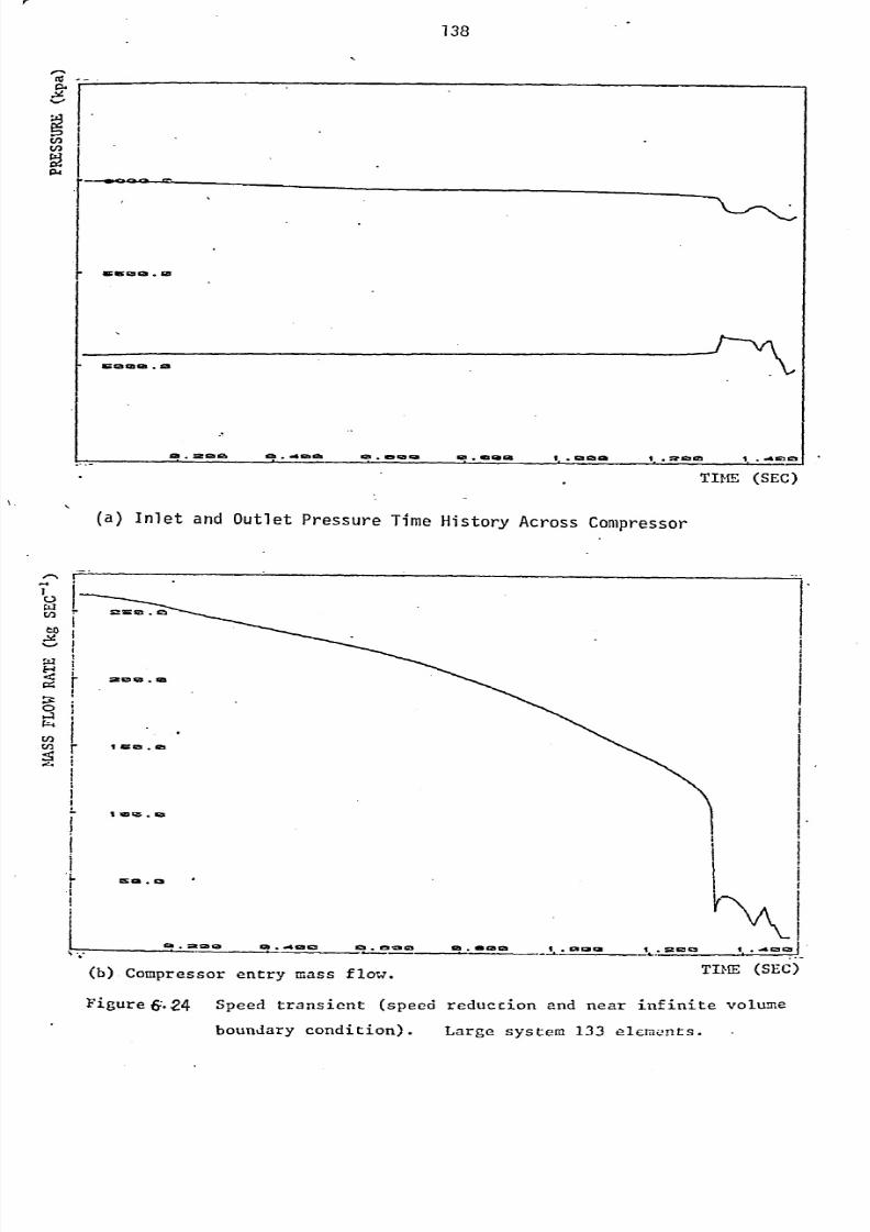
8/6/2019 A. M. Y. Razak Thesis 1984
http://slidepdf.com/reader/full/a-m-y-razak-thesis-1984 152/181
V
138
00404a
volmialmso
a lagagal. sa
ce . zecm 12. fe.. im . miaim 9. imcnica t. r%aCib 1. :eCN b--
lý . -4=] CN
TIME (SEC)
(a) Inlet and Outlet Pressure Time History Across Compressor
I-
r
a lagagal. sa
I In tr, . la
1. -4 CB cm ga.
9!! e= CN da.m
ga la t. ga cm cm 1 usi5cs 1. -6 c234b
(b) Compressor entry mass flow. TIME (SEC)
Figure 6.24 Speedtransient
(speedreduccion and near
infinitevolume
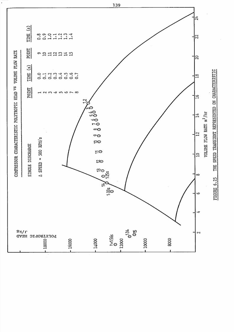
8/6/2019 A. M. Y. Razak Thesis 1984
http://slidepdf.com/reader/full/a-m-y-razak-thesis-1984 153/181
139
Ln
cqQ;
Hrm4
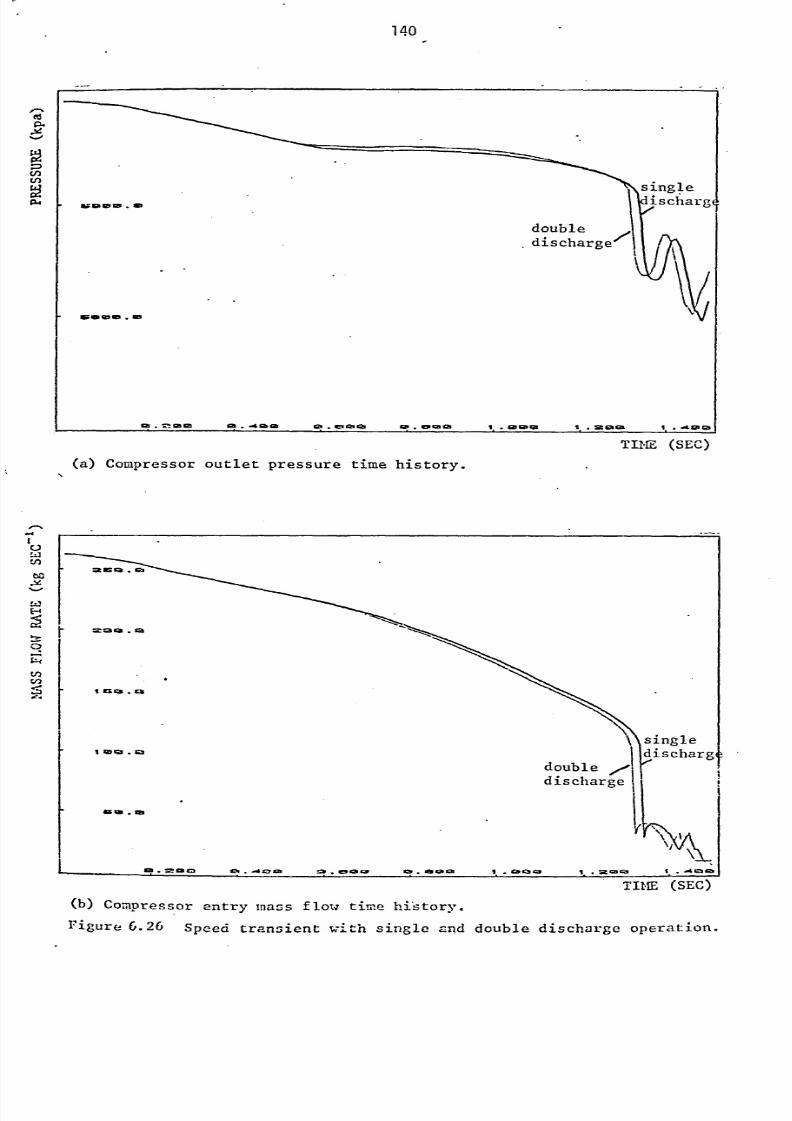
8/6/2019 A. M. Y. Razak Thesis 1984
http://slidepdf.com/reader/full/a-m-y-razak-thesis-1984 154/181
p.
1-11
cis.
it im la 929. -4 Gb a lot . es al 12, R. Im ch 121 1. CD cal 01 1. mcgGeL I. .4 ja ra.
TIME (SECI)
(a) Compressor outlet pressure time history.
0
AN& as
V'I'
'A'
ge. 2. a ca ice. 14 931m
-e . e! aGip Cb to imca ýý. cac3,43 ý. .a ca 23--1. . -4G3 a
TIME (SEC)
(b) Compressor entry inass f low time hi'story.
rigure 6.26
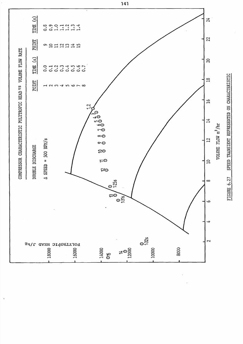
8/6/2019 A. M. Y. Razak Thesis 1984
http://slidepdf.com/reader/full/a-m-y-razak-thesis-1984 155/181
141
C14CN
0C14
00,4
1-4
-zr
r-I
0
OD
'.0
-T
C14
rý
TZ4
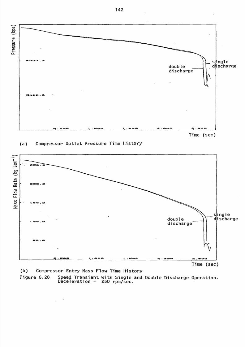
8/6/2019 A. M. Y. Razak Thesis 1984
http://slidepdf.com/reader/full/a-m-y-razak-thesis-1984 156/181
142
(dCL
1.2-j
(1)
nglescharge
0. WOO I. gaGa a I. moca =. 12gala :a. ISO szl
Time (sec)
(a) Compressor Outlet Pressure Time History
V)
En
4-3M5
0r-LL-
Ln(n
im xaKiNla
.= ases .0
=OCB.
an
Iar ca . am
I saa . ca
292A
.
ga
doubledischarge
\t
1. . gagaca 1. . 990 IM ta 421a ISIM12i
ýngl escharge
Time (sec)
(b) Compressor Entry Mass Flow Time History
Figure 6.28 Speed Transient with Single and Double Discharge Operation.Deceleration = 250 rpm/sec.
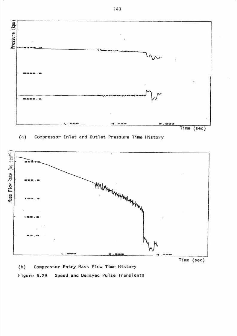
8/6/2019 A. M. Y. Razak Thesis 1984
http://slidepdf.com/reader/full/a-m-y-razak-thesis-1984 157/181
143
C6ca.
ci,
t/)
a,
ir. Es GDGD. im
moosa . G5
1,. 65010 =ý. so-
m! .00 la
(a) Compressor Inletand
Outlet Pressure Time History
a)
I
I lasm la
1521
.M
t. la 123 0
'V
F. valmal :!!!-.
%azas
Time (sec)
Time (sec)
(b) Compressor Entry Mass Flow Time History
Figure 6.29 Speed and Delayed Pulse Transients
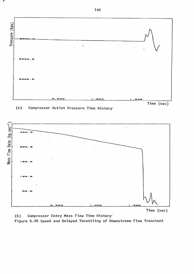
8/6/2019 A. M. Y. Razak Thesis 1984
http://slidepdf.com/reader/full/a-m-y-razak-thesis-1984 158/181
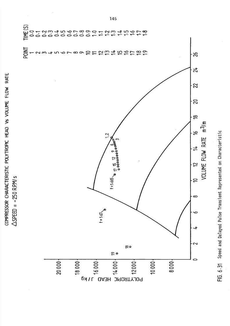
8/6/2019 A. M. Y. Razak Thesis 1984
http://slidepdf.com/reader/full/a-m-y-razak-thesis-1984 159/181
LO
!acc
SLi-
LLJ
0IA
X:a:clýC>Ln
C14I
11
ClU-iLLJa-V)
145
UJ C? '7 Cý4l? Lf? '9 r'ý' C? Cý'
C:> 4=>CD C:: C:: C) C) CD
COv-
c,4 rn t Ln
%. r-- oo (7, cD clJm Ln I V-cc) C7%
Q_
C)CD
CDC%4
T-I-i I-: I-L V--V- V-: T-LV-:
C=) C>
Cýp
C1.4
V-qr-
5ý/r OV3HDIdOdi)00d
c, 4 m Ln .o r- co
CDCDP C>
CC)
CY)
E
CD
-iLL
LLJ
C)
tnr_fli
-ci
ccir-ai
cm
-ci
r_-
T-m
U3LL
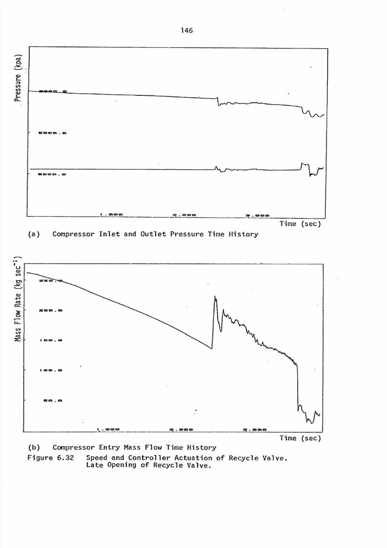
8/6/2019 A. M. Y. Razak Thesis 1984
http://slidepdf.com/reader/full/a-m-y-razak-thesis-1984 160/181
146
A:
CL)
IAV)
ir. Miaim. Na
esma c23
. im
1.12)v CB
gal aa gala 0
(a) Compressor Inlet and Outlet Pressure Time History
U
4-3
0
r-LL-
w
t/Y
2.
Time (sec)
Time (sec)
(b) Compressor Entry Mass Flow Time History
Figure 6.32 Speed and Controller Actuation of Recycle Valve.Late Opening of Recycle Valve.
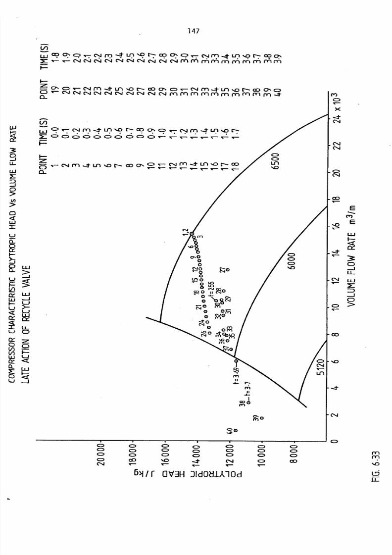
8/6/2019 A. M. Y. Razak Thesis 1984
http://slidepdf.com/reader/full/a-m-y-razak-thesis-1984 161/181
147
:ZCDF--Li
LU
U. c9 cý, c:? ý-7 c, ý m -t uý '-9 t-ý Ci? oý C? 7 rg rý -4 L12 0 C-ý- CK?cý,2: N- r- C'4 C, C%4C'4 CN C'4 CN C*ýj C, j CN MMmMmmmmMm
F-
F--ý
C*4M -t Lfl %0 t- OD CY% ) l'r- C4 M -. Lrl %M - CO CY%Dc*-i C-4 c, 4 C,i
C, C-4 cý4 c-4 c,4 mmmmMmmMMmt2-
cl%
MG
C)ýo
It
cý cý> cý cý C: )CD c> CD C> (D (D CD
CD CD C> CD C) C> CDC: ) CD %D
-t c44 C> CoCI-4 %- 19-- e- Ir- Ir-
CY)C)T-x
ýtC14
CN0*4
CN
CC)T-
%DIr-
ý 1t
C14
h OD
%0
-t
C4
E
cnE
LU
C:
-ii-
LUZ
CD
6W OV3HDIdOdD,0d
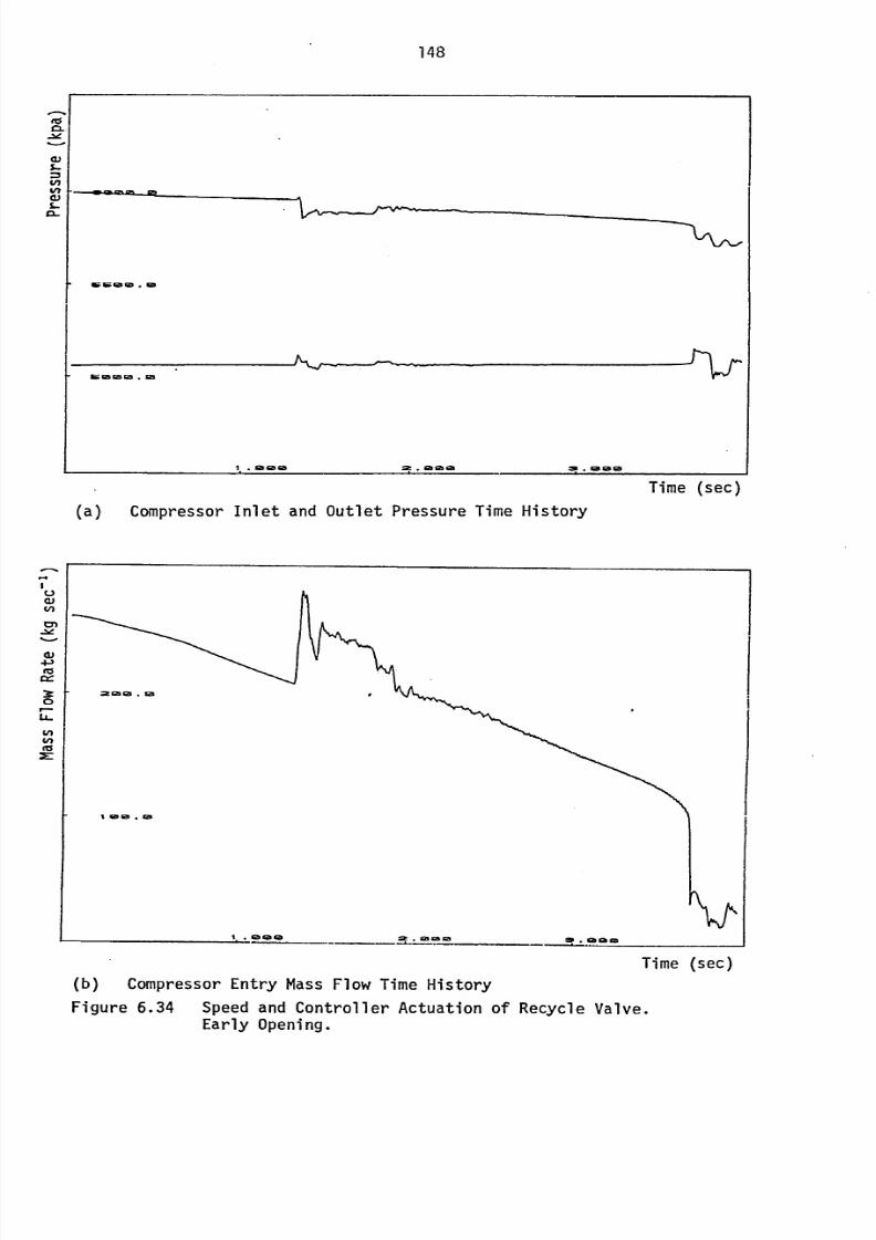
8/6/2019 A. M. Y. Razak Thesis 1984
http://slidepdf.com/reader/full/a-m-y-razak-thesis-1984 162/181
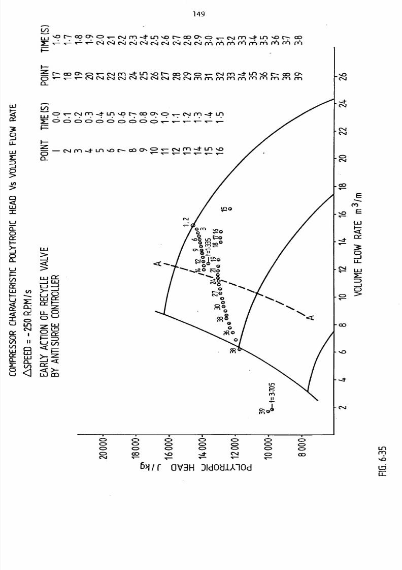
8/6/2019 A. M. Y. Razak Thesis 1984
http://slidepdf.com/reader/full/a-m-y-razak-thesis-1984 163/181
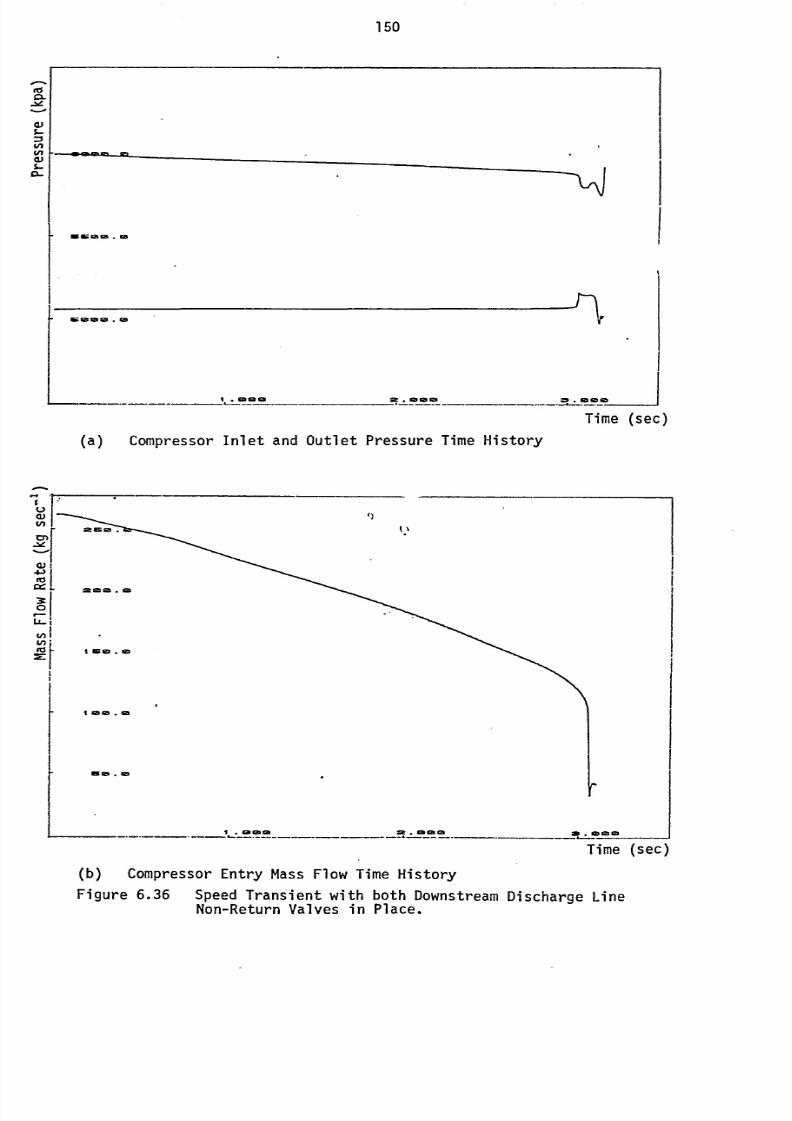
8/6/2019 A. M. Y. Razak Thesis 1984
http://slidepdf.com/reader/full/a-m-y-razak-thesis-1984 164/181
150
ildL
d)S-CL
mw. Caim . Na
woolm. Gb
11
I
I.Moo Zt. laimo M. laosm
Time (sec)
o-ý
(a) Compressor Inlet and Outlet Pressure Time History
1daimgib
We. in
.-m.IMCNCN
Time (sec)
(b) Compressor Entry Mass Flow Time History
Figure 6.36 Speed Transient with both Downstream Discharge LineNon-Return Valves in Place.
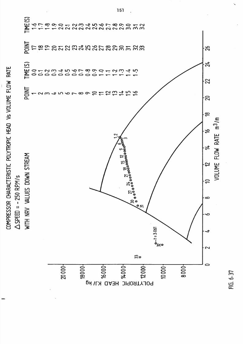
8/6/2019 A. M. Y. Razak Thesis 1984
http://slidepdf.com/reader/full/a-m-y-razak-thesis-1984 165/181
151
ui r- co C7.,:> ý, " rn 't Ln 'o r- co C7.,:v-*- ,- t-*- 0: 4 C-4 C44 C-ý C-ý C-ý C--: 0: 4 C-ý Clý r6
I-
r- co a, p ý, c,4
rn -tLn o r- a: ) a, c=) , cN m
CD -- v- " C'14C14 C1404 04 (N " CN MM rn MCL
%0
h14
E
cY,
E
Ln
C)LLJLLJa-
rnMO
CD CD
(Z) C)CD ODC,4 Ir-
CD CD C>C> C) CDCD C: ) CD
%D 't CN
Ir-Ic-
CDCD(Z)
Co
C)
LLJ
C)-jL
LLJ
CD
N Of OV3H IdOdl)Md
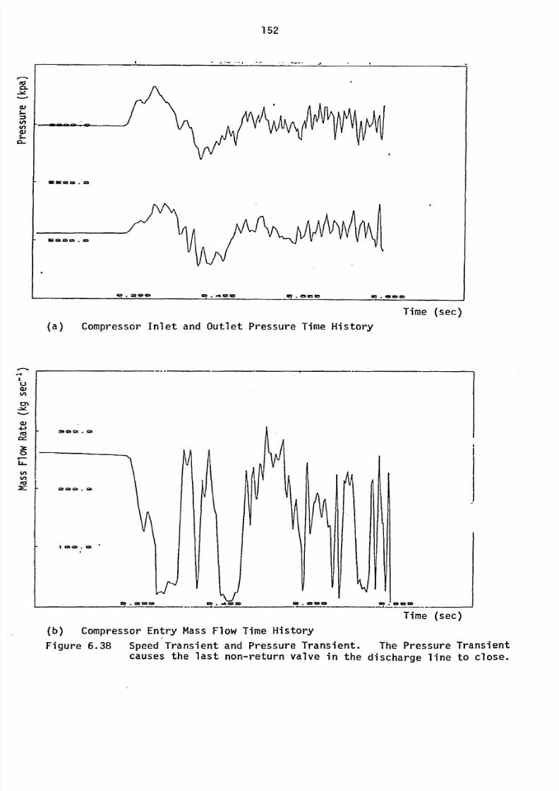
8/6/2019 A. M. Y. Razak Thesis 1984
http://slidepdf.com/reader/full/a-m-y-razak-thesis-1984 166/181
152
j
0-
CA4NMINOW26--40
inZ im a ica
Jr. GNa ON . 921
_15.mae. 42ý. .4 im 11D
'm
/VVW
I
IN
I
IV45195 gal lip
.aaes
Time (sec)
uM
W4-3fts
C4
3:0
LL-
(a) Compressor Inlet and Outlet Pressure Time History
Mp 95 la .ca
st saga .rb
1ca m,la ,
I
ib. ze 123 91 ims .ý miD M
i
II
LJ
I
I
ACD
gs, Go m
h
I
I
1ýI
I
Time (sec)
(b) Compressor Entry Mass Flow Time History
Figure 6.38 Speed Transient and Pressure Transient. The Pressure Transient
causes the last non-return valve in the discharge line to close.
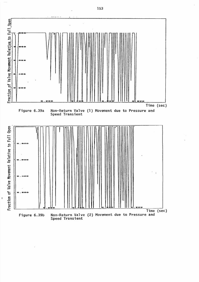
8/6/2019 A. M. Y. Razak Thesis 1984
http://slidepdf.com/reader/full/a-m-y-razak-thesis-1984 167/181
153
w
N-
lopolm
eslow
zenD
I
-4 IMN a
Im
WCL
CD
I-
U-
04)
w>
4)
I-
13in Gý G3
ra . e5 ca ca
4-3
E
0x
W
4-0
00
4-3
LL-
ga .41310
Ch=oo
121.01210
Ti
10
A
I
11
6. ek66
I
Rj9wr! al
Time (sec)
Figure 6.39b Non-Return Valve (2) Movementdue to Pressure andSpeed Transient
rm
I
I
Gý.Z 1250
11
ni
I
IV
I
xi? IF V a
Time (sec)
Figure 6.39a Non-Return Valve (1) Movementdue to Pressure andSpeed Transient
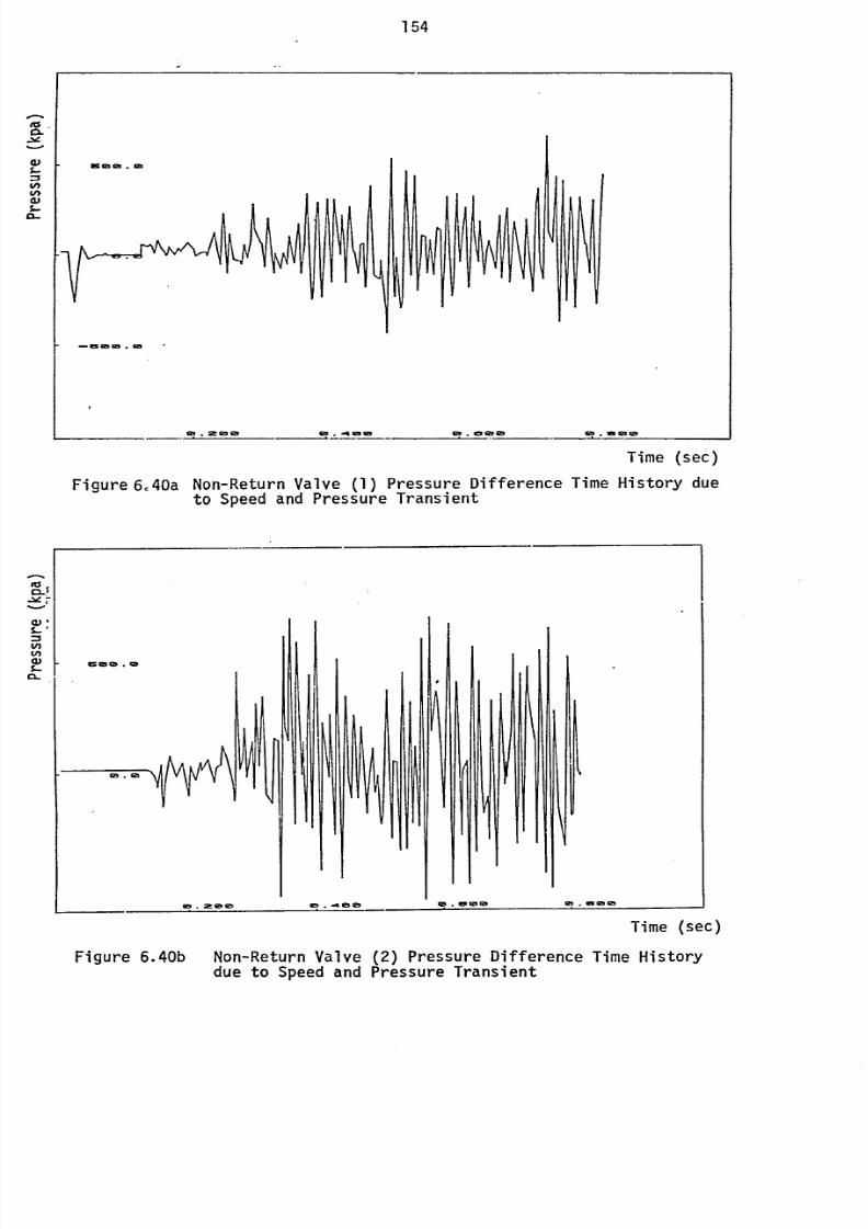
8/6/2019 A. M. Y. Razak Thesis 1984
http://slidepdf.com/reader/full/a-m-y-razak-thesis-1984 168/181
154
w95
O.
65
-iscsm.w
p
I
I
I I
I HýI
I
1
kol
0
I
I
I
I I I
N1
1; .= C23l es . -4 m 95 in .0 es G5 Gý . in Q50
Time (sec)
Figure 6,40a Non-Return Valve (1) Pressure Difference Time History dueto Speed and Pressure Transient
moo . Op
ia . la
I
11
11
ý, I
I
11
ýj
I
I
II
III
I
I
I
I
I
115ý 0 la %g . 400 la
.151 m ID e?
.oa3 Cb
Time (sec)
Figure 6.40b Non-Return Valve (2) Pressure Difference Time Historydue to Speed and Pressure Transient
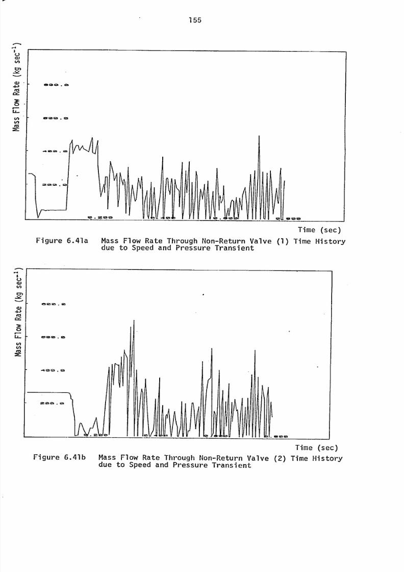
8/6/2019 A. M. Y. Razak Thesis 1984
http://slidepdf.com/reader/full/a-m-y-razak-thesis-1984 169/181
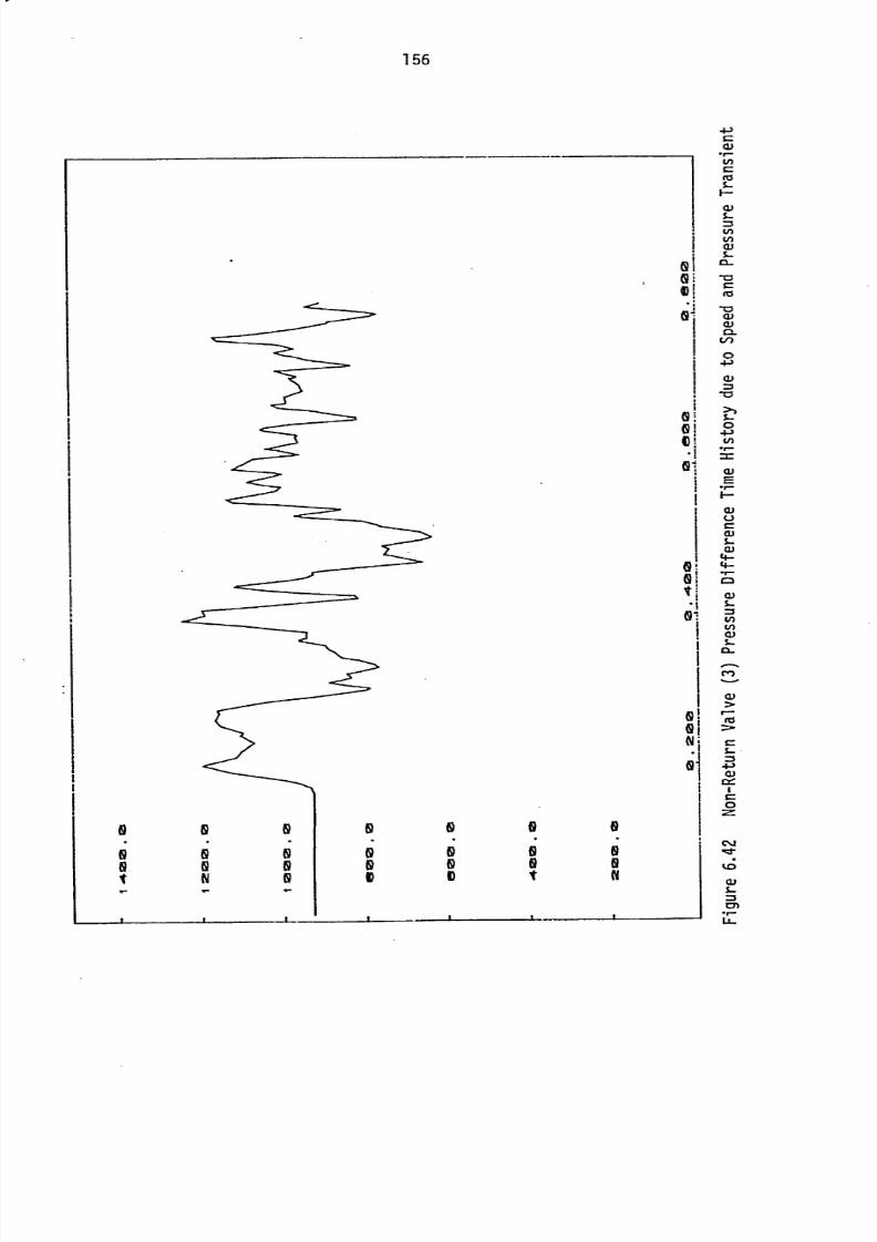
8/6/2019 A. M. Y. Razak Thesis 1984
http://slidepdf.com/reader/full/a-m-y-razak-thesis-1984 170/181
156
4-)
S-
-0r-ms
-0a)CL)CLV)
0
-0
o4-3
F-
WUC
cuS-
a)4-4-
r-CM
a)
CY)
4-3
0
C14i-d-
M. r.LL.
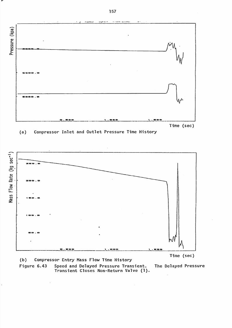
8/6/2019 A. M. Y. Razak Thesis 1984
http://slidepdf.com/reader/full/a-m-y-razak-thesis-1984 171/181
157
OL
4b4h
q
L
IN lw ca ca . ca
e Cb m 0. im
! ý_. 1.. MCMID
-r--
I.is G5 ca
(a) Compressor Inlet and Outlet Pressure Time History
go
0f-LL-
st scaIn
sen MGb
I Iscm. la
1mr5 . in
e CB. ja
1. . on cm
Time (sec)
w
Time (sec)(b) Compressor Entry Mass Flow Time History
Figure 6.43 Speed and Delayed Pressure Transient. The Delayed Pressure
Transient Closes Non-Return Valve (I).
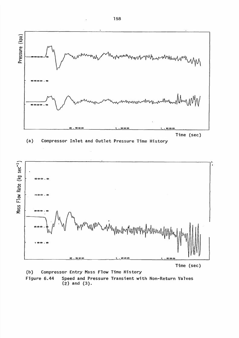
8/6/2019 A. M. Y. Razak Thesis 1984
http://slidepdf.com/reader/full/a-m-y-razak-thesis-1984 172/181
158
cu
L-
cuS-
fl-
Time (sec)
(a) Compressor Inlet and Outlet Pressure Time History
L)
M
ci4-)
U-
UQ G3.
G3
-4 Q 92. .0
m. gar! ' . %Z,
ý130
IG!, ca .0
Ge . r. Gb ex lý. im ia c!N
I. 0.4a Q
I
I
I
r
Time (sec)
(b) Compressor Entry Mass Flow Time History
Figure 6.44 Speed and Pressure Transient with Non-Return Valves(2) and (3).
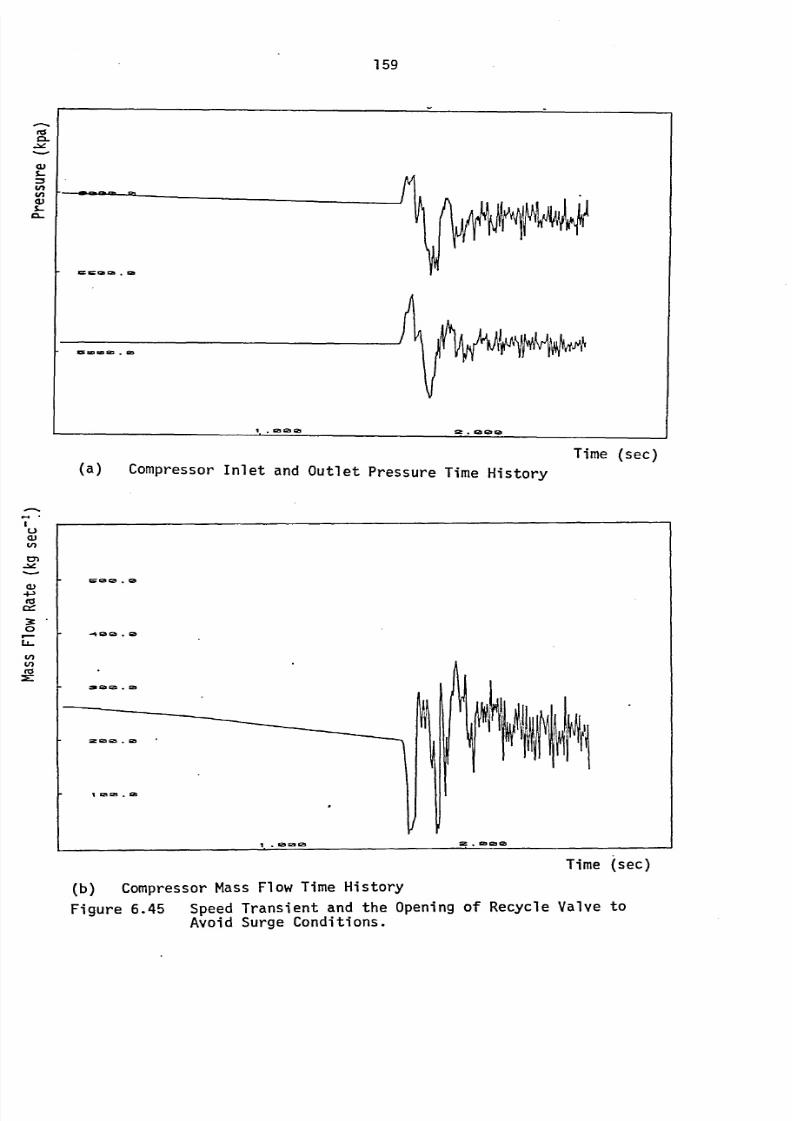
8/6/2019 A. M. Y. Razak Thesis 1984
http://slidepdf.com/reader/full/a-m-y-razak-thesis-1984 173/181
159
. -I
cU
CL
S-
(A(A
uV(n
C)
4-3co
Of
31 ,0
LL.
WV)co
X:
=a smm925
1ima im rs
.m
1.. 121 b Gb
mjppýow,ýv
Mýlo
:;ý * ca 0 ca
(a) Compressor Inlet and Outlet Pressure Time History
ý ca ca . 10
.40 Gb . lib
2DD22. rb
0121C21.
Gb
I so=&B
9b2112%
I
iI1 10,
Time (sec)
f
zewm mm
Time (sec)
(b) Compressor Mass Flow Time History
Figure 6.45 Speed Transient and the Opening of Recycle Valve toAvoid Surge Conditions.
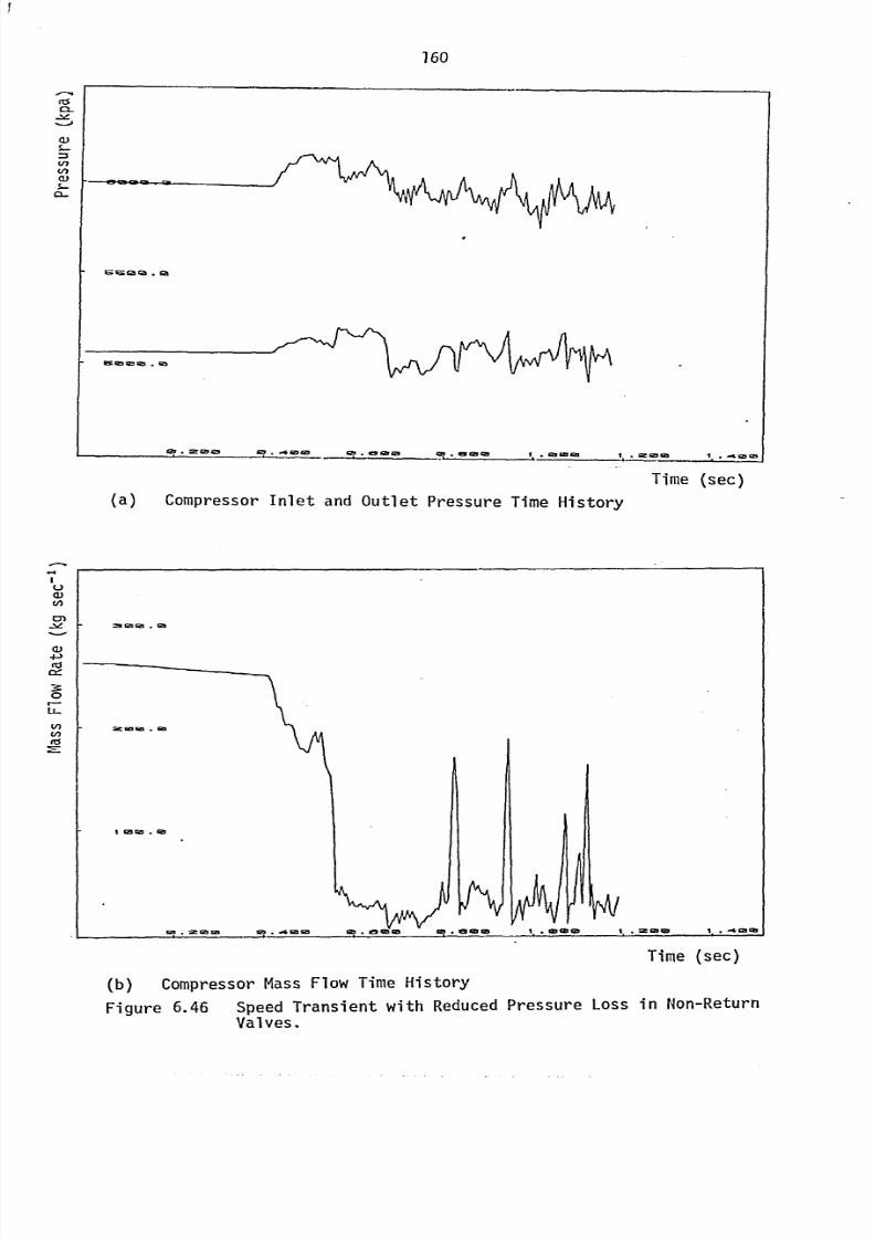
8/6/2019 A. M. Y. Razak Thesis 1984
http://slidepdf.com/reader/full/a-m-y-razak-thesis-1984 174/181
160
M-
-2z-. i
I
M. 1-. G! Q%. G6
wa Q2 Sal
. la
121 .= 12Pg
rAm
223 . ý4 da 93 42ý . c* darm 122923 ga
I
1. . Zz GM0 1.. -4 AM12%
Tinie (sec)
ei(n
cn
-2.
tii
LL-
0cn
(a) Compressor Inlet and Outlet Pressure Time History
29 aa . ca
GEo sm . Gm
I
JGIs G3 so ED cl) I& Im us .a
GM GS 05 121 sm 171
Time (sec)
1ar3 .
la
(b) Compressor Mass Flow Time History
Figure 6.46 Speed Transient with ReducedPressure Loss in Non-Return
Valves.
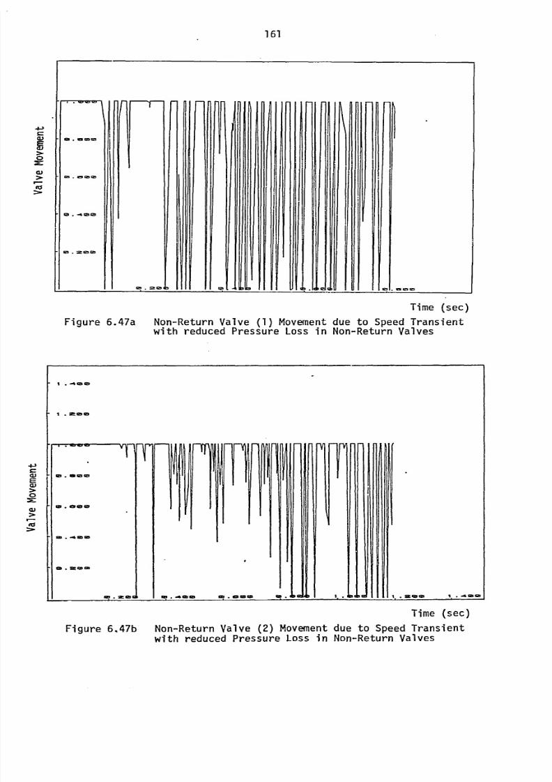
8/6/2019 A. M. Y. Razak Thesis 1984
http://slidepdf.com/reader/full/a-m-y-razak-thesis-1984 175/181
161
sow Go o
iCB
e3 923Gl.
0-49so
la .m r5 ca
rlF--T-l
-S-Wý
I I
I
ib
II
I I
I
ell. a Qq a
Time (sec)
Figure 6.47a Non-Return Valve (1) Movement due to Speed Transientwith reduced Pressure Loss in Non-Return Valves
r* I. -4 95 lb
I. Mlaw
ITfl93. miacv
im 0043
9D .16 D m
Gb
.
sc =In
T. %aa
n
e! . -4Cba c? . dmmw
m
II
I
t.1111
I
lit
1. . me so NZI 1. . .4 CD Qb
Time (sec)
Figure 6.47b Non-Return Valve (2) Movementdue to Speed Transient
with reduced Pressure Loss in Non-Return Valves
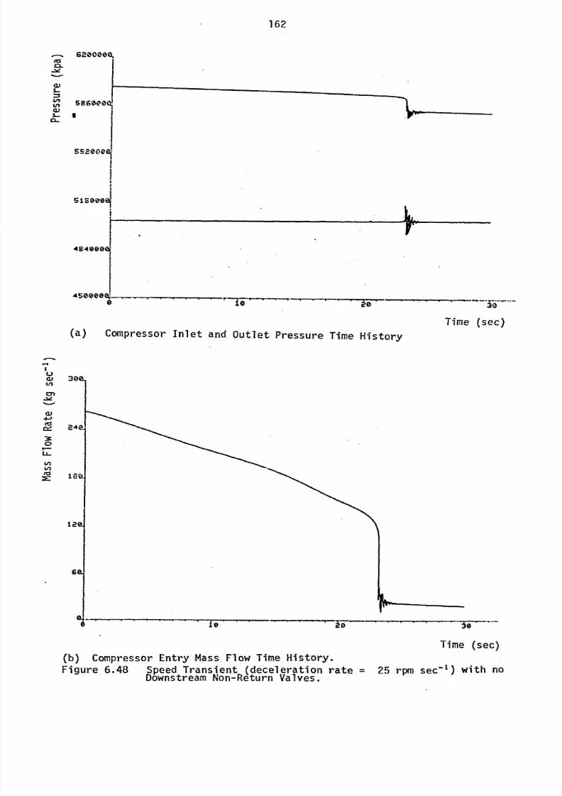
8/6/2019 A. M. Y. Razak Thesis 1984
http://slidepdf.com/reader/full/a-m-y-razak-thesis-1984 176/181
162
CL
ID- 1
552000a
slsooeý
4840006
45eeeee r-T äe- .-. ---. W,
Time (sec)(a) compressor Inlet
andOutlet Pressure
Time History
L)
W4-)tz
0-1
LL.V)W
30CL
2401
Israj
IM
Sk
T170
Time (sec)
(b) Compressor Entry Mass Flow Time History.
Figure 6.48 SDeedTransient (deceleration rate = 25 rpm sec-1) with noD6wnstreamNon-Return Valves.
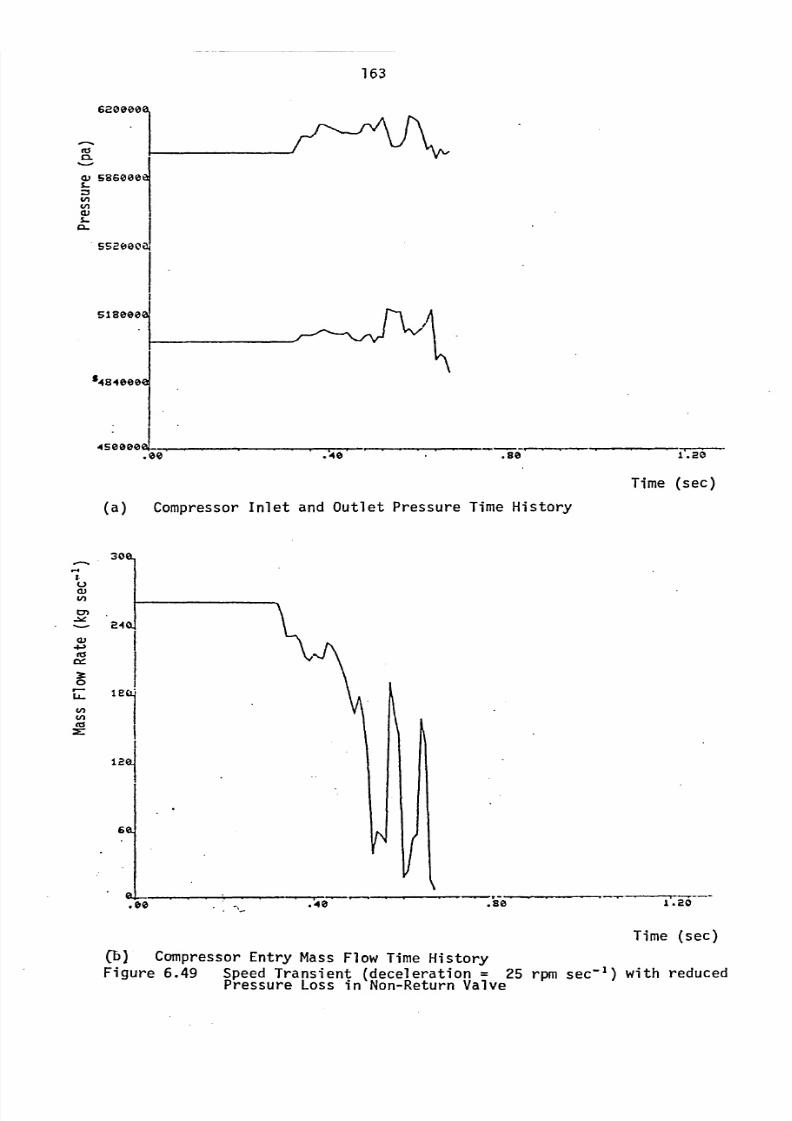
8/6/2019 A. M. Y. Razak Thesis 1984
http://slidepdf.com/reader/full/a-m-y-razak-thesis-1984 177/181
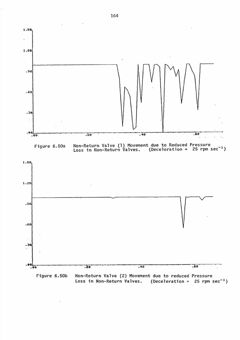
8/6/2019 A. M. Y. Razak Thesis 1984
http://slidepdf.com/reader/full/a-m-y-razak-thesis-1984 178/181
164
1.5ý
1. M
. gej
. 6(C N
I. 3eý
I
.40 60
Figure 6.50a Non-Return Valve (1) Movementdue to Reduced Pressure
Loss in Non-Return Valves. (Deceleration = 25 rpm sec-1)
1.5ý
1.21
. C4al
. 6a
. 30J
.e0 420
I
. 40
r--ýV-
I
. 613
Figure 6.50b Non-Return Valve (2) Movementdue to reduced Pressure
Loss in Non-Return Valves. (Deceleration = 25 rpm sec-')
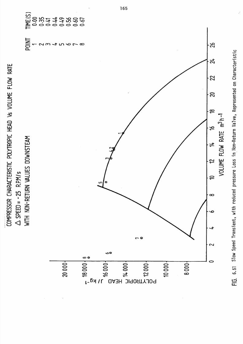
8/6/2019 A. M. Y. Razak Thesis 1984
http://slidepdf.com/reader/full/a-m-y-razak-thesis-1984 179/181
uj!ýi
CE-1
9U-
LLJ
0
165
LnC> Ln
CY,0 C) t--U (D ry) ýt t Lri%0 %.
CD C> C: ) C> C> C) IC::
F-:21-116 v- c-4 Ln %o - cc)la-
r- 0
cc) 0'oe
C) C=) C> CDC> CD C> CD
C) C) C=) C) C)
C=> OD %004 Ir", vl-
L-bmr OV3HDIdOdi),Od
%D
Flý4
04C'14
0
4-3u
C0
-aa)4-)
CN
CL)
Co
%D
ý --t
t"
C)
>r-CY)
E
LIJ S-=3-)Cl)
L=I
CD -11
-i r_ ,
LU
x:
CD
CLV)
ý1:0
r-
V)
tA(A0
Ln(A
Q.
-0Q)L)
:3_0cu
4J
4-;
(o
Lf)
kjý
LOLL-
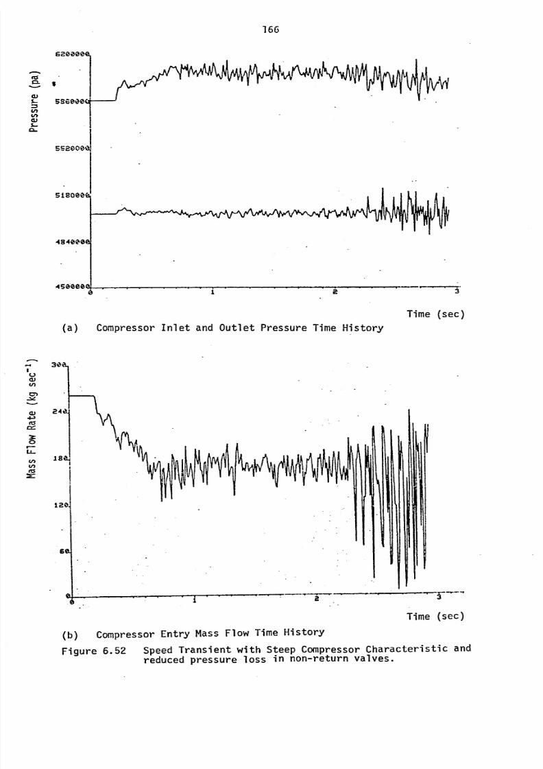
8/6/2019 A. M. Y. Razak Thesis 1984
http://slidepdf.com/reader/full/a-m-y-razak-thesis-1984 180/181
166
6200M.
I'dCL
cu
fl-
SE-21DOOJ
Time (sec)
L)
cr-
3::0
LL-
Ln
V)
(a) Compressor Inlet and Outlet Pressure Time History
120
sc,
I
I
a
Time (sec)
(b) Compressor Entry Mass Flow Time History
Figure 6.52 Speed Transient with Steep Compressor Characteristic and
reduced pressure loss in non-return valves.
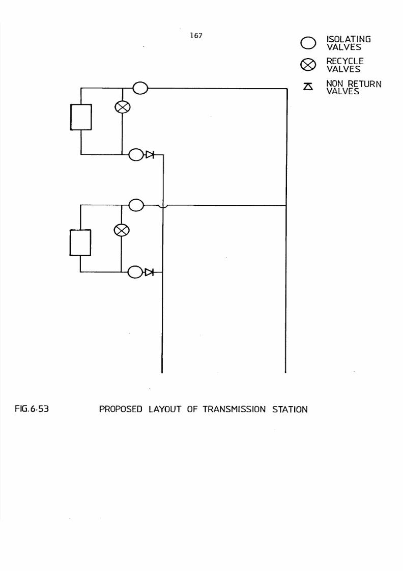
8/6/2019 A. M. Y. Razak Thesis 1984
http://slidepdf.com/reader/full/a-m-y-razak-thesis-1984 181/181
1670 ISOLATING
VALVES
RECYCLEVALVES
zs NONRETURNVALVES


![Full Thesis[1]](https://static.fdokumen.site/doc/165x107/54e518aa4a7959657e8b462a/full-thesis1.jpg)