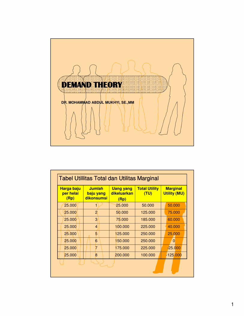
1

DEMAND THEORYDEMAND THEORYDEMAND THEORYDEMAND THEORYDEMAND THEORYDEMAND THEORYDEMAND THEORYDEMAND THEORY

DR. MOHAMMAD ABDUL MUKHYI, SE.,MM

Tabel Utillitas Total dan Utilitas MarginalTabel Utillitas Total dan Utilitas Marginal

Harga baju per helai

(Rp)

Jumlah baju yang

dikonsumsi

Uang yang dikeluarkan

(Rp)

Total Utility (TU)

Marginal Utility (MU)

25.000 1 25.000 50.000 50.000

25.000 2 50.000 125.000 75.000

25.000 3 75.000 185.000 60.000

25.000 4 100.000 225.000 40.000

25.000 5 125.000 250.000 25.000

25.000 6 150.000 250.000 0

25.000 7 175.000 225.000 -25.000

25.000 8 200.000 100.000 -125.000

2

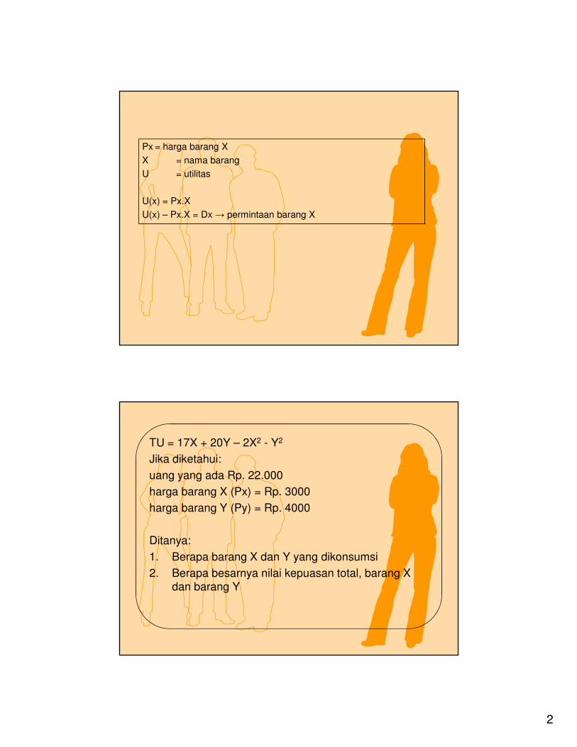
Px = harga barang X

X = nama barang

U = utilitas

U(x) = Px.X

U(x) – Px.X = Dx → permintaan barang X

TU = 17X + 20Y – 2X2 - Y2

Jika diketahui:

uang yang ada Rp. 22.000

harga barang X (Px) = Rp. 3000

harga barang Y (Py) = Rp. 4000

Ditanya:

1. Berapa barang X dan Y yang dikonsumsi

2. Berapa besarnya nilai kepuasan total, barang X

dan barang Y

3

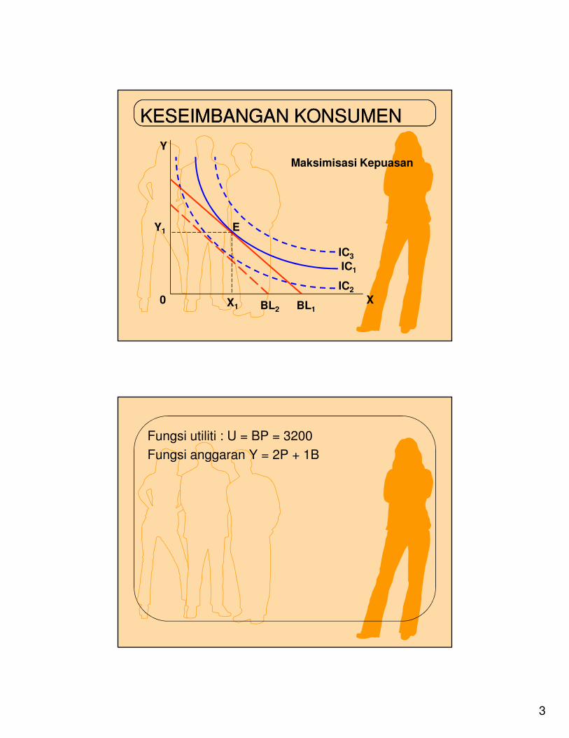
KESEIMBANGAN KONSUMENKESEIMBANGAN KONSUMEN

Y

0 X

E

IC2

IC1

IC3

BL2 BL1

Y1

X1

Maksimisasi Kepuasan

Fungsi utiliti : U = BP = 3200

Fungsi anggaran Y = 2P + 1B

4

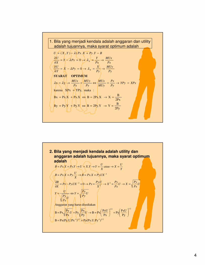
1. Bila yang menjadi kendala adalah anggaran dan utility

adalah tujuannya, maka syarat optimum adalah

2Py

B Y 2Py.Y B Py.Y Py.Y By

2Px

BX 2Px.X B Px.X Px.X Bx

:maka YPy, XPx karena

y x

0

0

..(),(

=→=⇔+=

=→=⇔+=

=

=→=⇔=→=

→=→=−=∂

∂

→=→=−=∂

∂

−+−=

XPxYPyPy

Px

MUy

MUx

Py

MUy

Px

MUx

Py

MUy

Py

XPyX

Y

U

Px

MUx

Px

YPxY

X

U

BYPyXPxYXU

X

X

λλ

λλ

λλ

λ

OPTIMUM SYARAT

2. Bila yang menjadi kendala adalah utility dan anggaran adalah tujuannya, maka syarat optimum adalah

2/11-2/11-

2/12/1

2

2

2

1

)Py(Px.U.Py )Px(Py.U.Px B

Py

PxUPy

Px

PyUPxB

Py

PxPy

Px

PyPx B

disediakan harus yangAnggaran

.0.

....

...

+=

+

=→+=

=⇔=

=→=→=→=−=∂

∂

+=→+=

=→=→=→+=

−

−

UU

UPy

PxY

UPx

Py

UY

UPx

PyXU

Px

PyX

X

UPyPxUXPyPx

X

B

UXPyXPxBX

UPyXPxB

Y

UXatau

X

UYYXUYPyXPxB

5

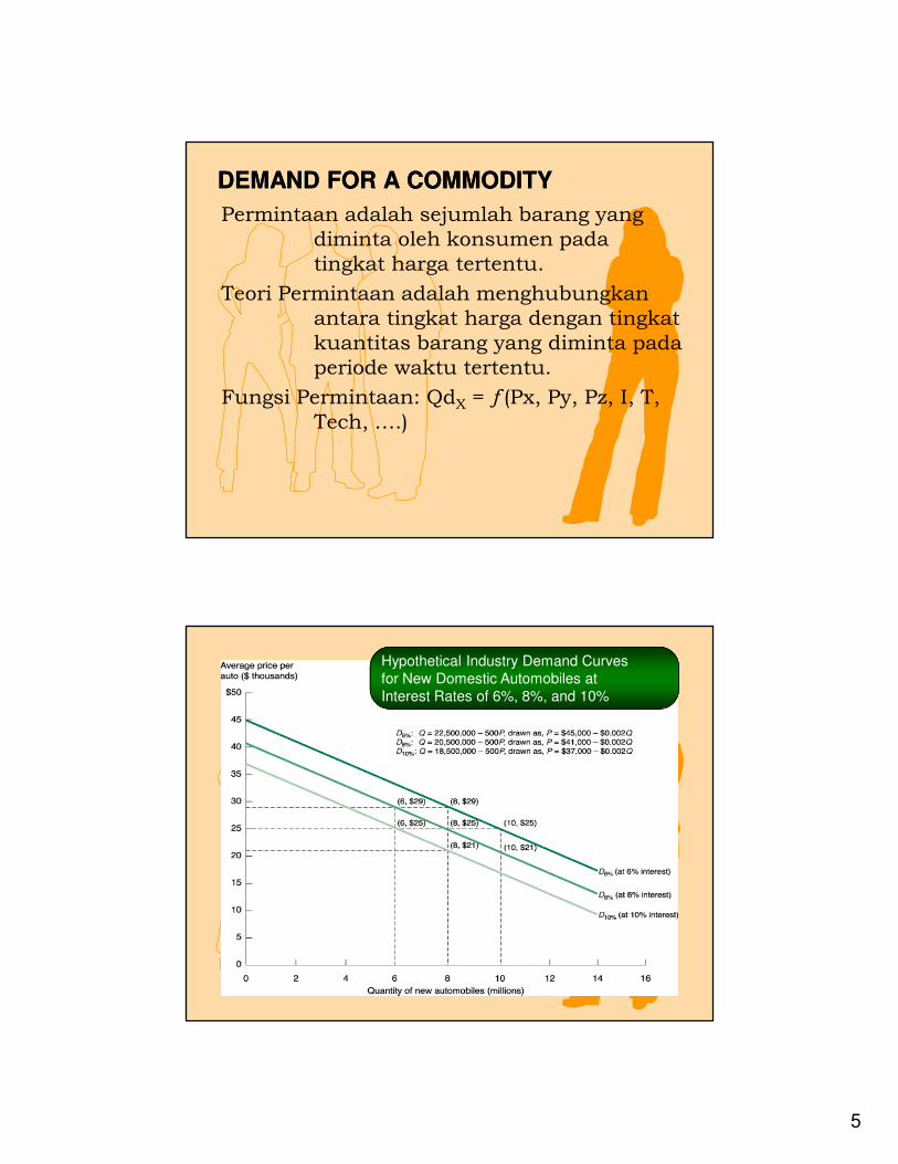
DEMAND FOR A COMMODITYDEMAND FOR A COMMODITY

Permintaan adalah sejumlah barang yang

diminta oleh konsumen pada

tingkat harga tertentu.

Teori Permintaan adalah menghubungkan

antara tingkat harga dengan tingkat

kuantitas barang yang diminta pada

periode waktu tertentu.

Fungsi Permintaan: QdX = ƒ(Px, Py, Pz, I, T,

Tech, ….)

Hypothetical Industry Demand Curves

for New Domestic Automobiles at

Interest Rates of 6%, 8%, and 10%

6

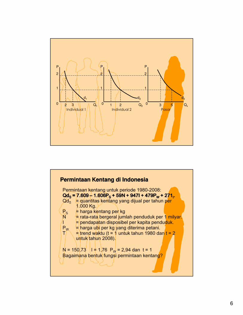
P

0 Q1

P P

Q2 Qx0 0

2 2 2

1 1 1

3 2 52 1 3

d1 d2 d3

Individual 1 Individual 2 Pasar

Permintaan Kentang di IndonesiaPermintaan Kentang di Indonesia

Permintaan kentang untuk periode 1980-2008:QdQdQdQdSSSS = 7.609 = 7.609 = 7.609 = 7.609 –––– 1.606P1.606P1.606P1.606PSSSS + 59N + 947I + 479P+ 59N + 947I + 479P+ 59N + 947I + 479P+ 59N + 947I + 479PWWWW + 271+ 271+ 271+ 271tttt....QdS = quantitas kentang yang dijual per tahun per

1.000 Kg.PS = harga kentang per kgN = rata-rata bergeral jumlah penduduk per 1 milyar.I = pendapatan disposibel per kapita penduduk.PW = harga ubi per kg yang diterima petani.T = trend waktu (t = 1 untuk tahun 1980 dan t = 2

untuk tahun 2008).

N = 150,73 I = 1,76 PW = 2,94 dan t = 1Bagaimana bentuk fungsi permintaan kentang?

7

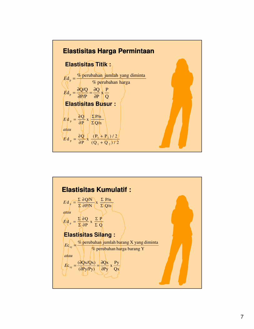
Elastisitas Harga PermintaanElastisitas Harga Permintaan

Elastisitas Titik :

Elastisitas Busur :

Q

P x

P

Q

P/P

Q/Qd

hargaperubahan %

diminta yangjumlah perubahan %d

p

p

∂

∂=

∂

∂=

=

E

E

2/)QQ(

2/)PP( x

P

Q d

Q/n

P/n x

P

Q d

21

21p

p

+

+

∂

∂=

Σ

Σ

∂

∂=

E

atau

E

Elastisitas KumulatifElastisitas Kumulatif ::

Q

P x

P

Q d

Q/n

P/n x

P/N

Q/N d

p

p

Σ

Σ

∂Σ

∂Σ=

Σ

Σ

∂Σ

∂Σ=

E

atau

E

Elastisitas Silang :

Qx

Py x

Py

Qx

Py/Py)(

Qx/Qx)(c

Y barang hargaperubahan %

diminta yang X barangjumlah perubahan %c

xy

xy

∂

∂=

∂

∂=

=

E

atau

E

8

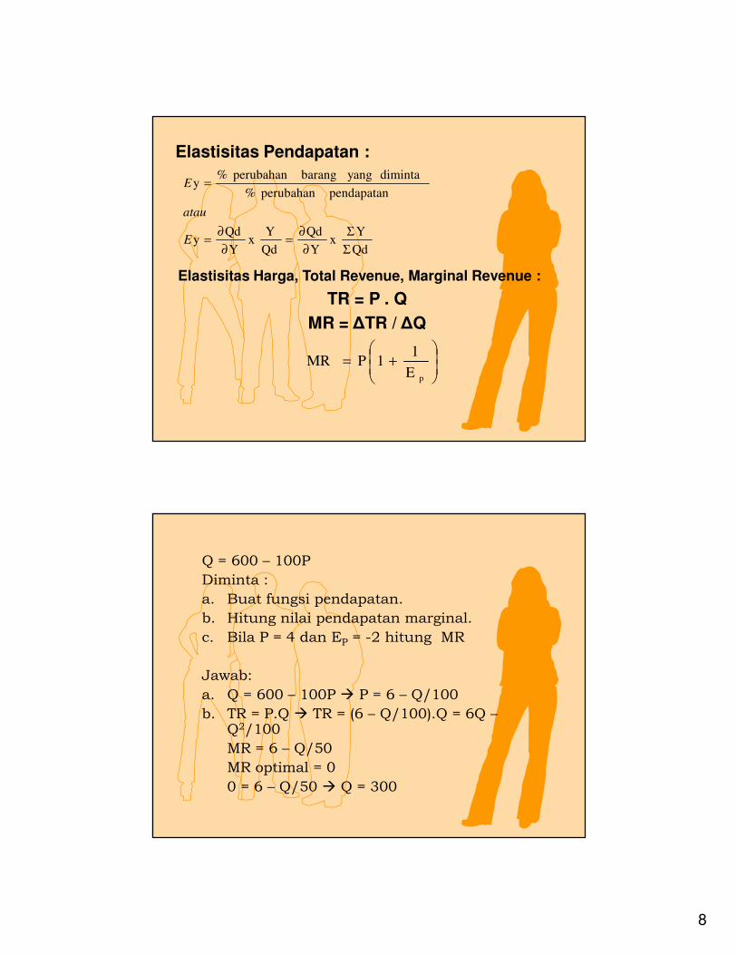
Elastisitas Pendapatan :

Qd

Y x

Y

Qd

Qd

Y x

Y

Qdy

pendapatanperubahan %

diminta yang barangperubahan % y

Σ

Σ

∂

∂=

∂

∂=

=

E

atau

E

Elastisitas Harga, Total Revenue, Marginal Revenue :

TR = P . Q

MR = ∆TR / ∆Q

+=

pE

1 1P MR

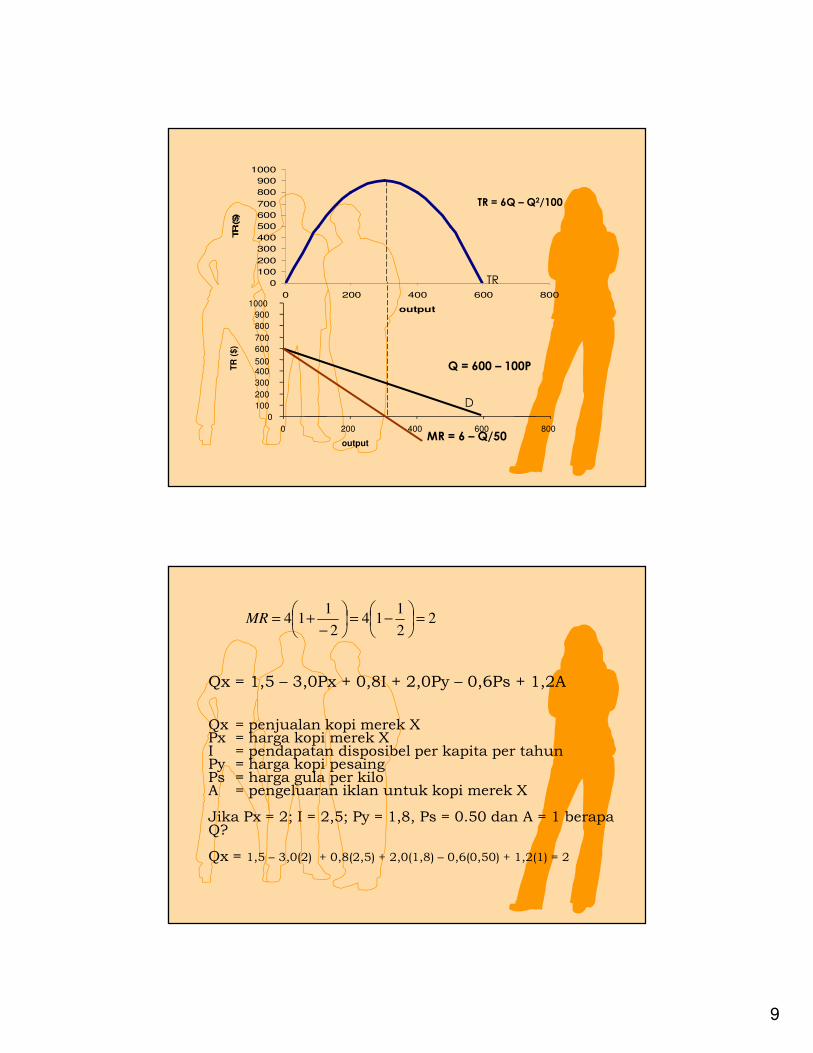
Q = 600 – 100P

Diminta :

a. Buat fungsi pendapatan.

b. Hitung nilai pendapatan marginal.

c. Bila P = 4 dan EP = -2 hitung MR

Jawab:

a. Q = 600 – 100P � P = 6 – Q/100

b. TR = P.Q � TR = (6 – Q/100).Q = 6Q –Q2/100

MR = 6 – Q/50

MR optimal = 0

0 = 6 – Q/50 � Q = 300

9

0

100

200

300

400

500

600

700

800

900

1000

0 200 400 600 800

output

TR ($)

TR

output

0

100

200

300

400500

600

700

800

900

1000

0 200 400 600 800

TR

($)

D

MR = 6 – Q/50

TR = 6Q – Q2/100

Q = 600 – 100P

22

114

2

114 =

−=

−+=MR

Qx = 1,5 – 3,0Px + 0,8I + 2,0Py – 0,6Ps + 1,2A

Qx = penjualan kopi merek XPx = harga kopi merek XI = pendapatan disposibel per kapita per tahunPy = harga kopi pesaingPs = harga gula per kiloA = pengeluaran iklan untuk kopi merek X

Jika Px = 2; I = 2,5; Py = 1,8, Ps = 0.50 dan A = 1 berapa Q?

Qx = 1,5 – 3,0(2) + 0,8(2,5) + 2,0(1,8) – 0,6(0,50) + 1,2(1) = 2

10

6,02

12,1E

15,02

50,06,0E

8,12

8,12E

12

2,50,8 E

32

23E

A

XS

XY

I

P

=

=

−=

−=

=

=

=

=

−=

−=

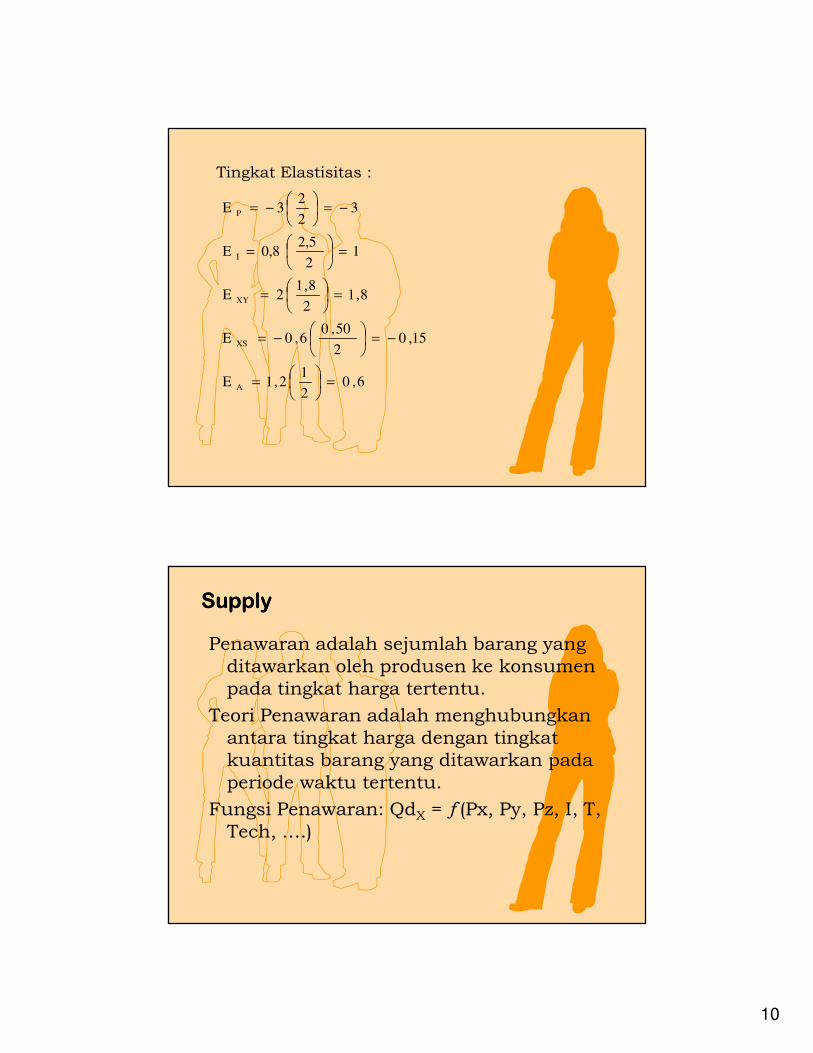
Tingkat Elastisitas :

SupplySupply

Penawaran adalah sejumlah barang yang

ditawarkan oleh produsen ke konsumen

pada tingkat harga tertentu.

Teori Penawaran adalah menghubungkan

antara tingkat harga dengan tingkat

kuantitas barang yang ditawarkan pada

periode waktu tertentu.

Fungsi Penawaran: QdX = ƒ(Px, Py, Pz, I, T,

Tech, ….)

11

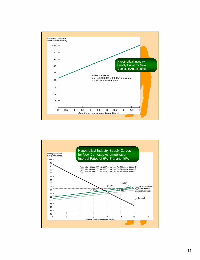
Hypothetical Industry

Supply Curve for New

Domestic Automobiles

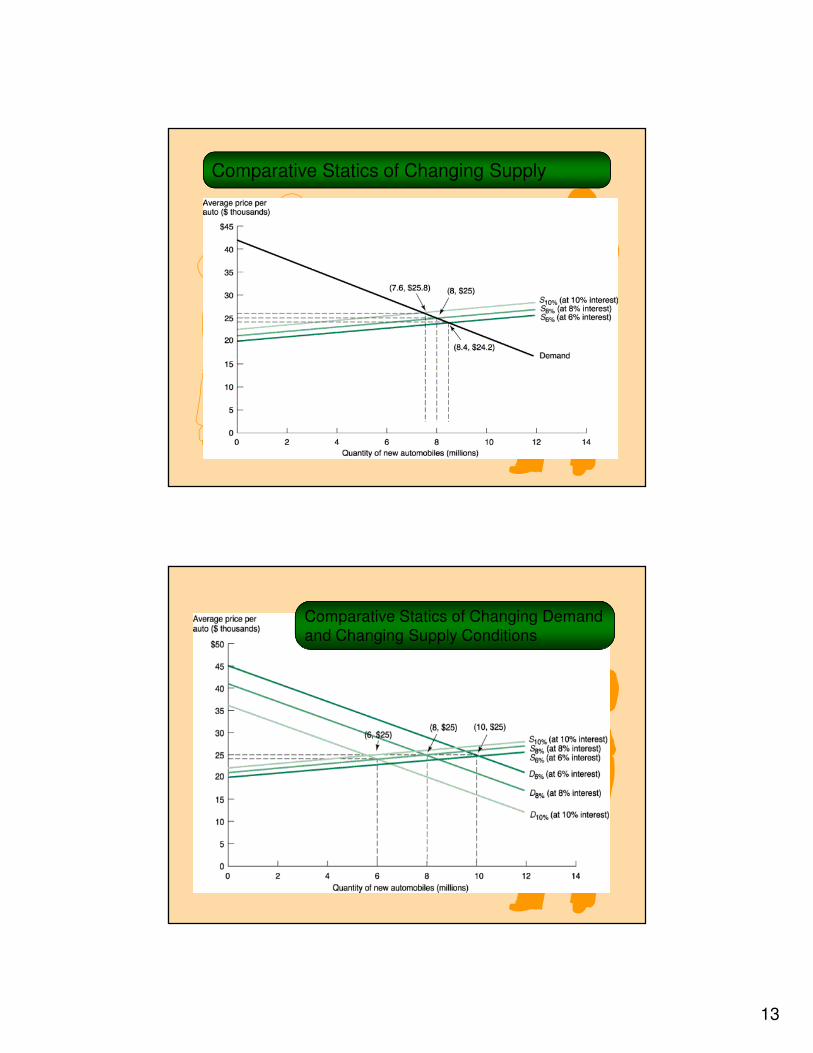
Hypothetical Industry Supply Curves

for New Domestic Automobiles at

Interest Rates of 6%, 8%, and 10%

12

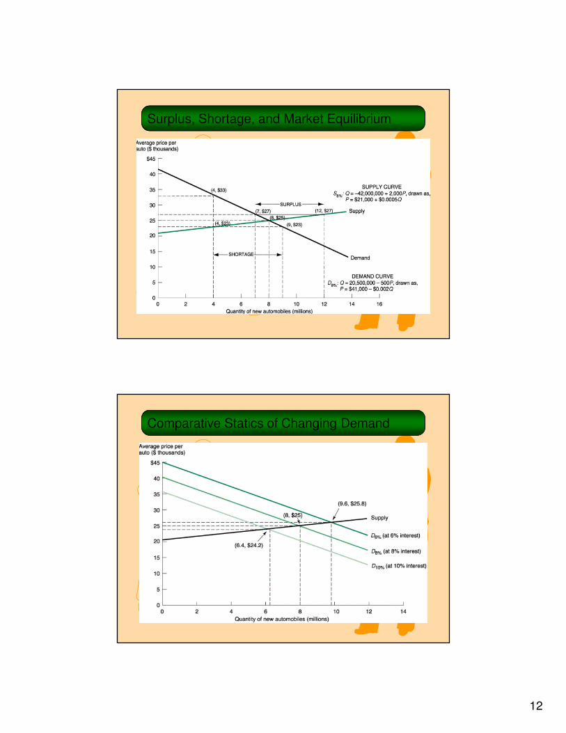
Surplus, Shortage, and Market Equilibrium

Comparative Statics of Changing Demand

13

Comparative Statics of Changing Supply

Comparative Statics of Changing Demand

and Changing Supply Conditions

14

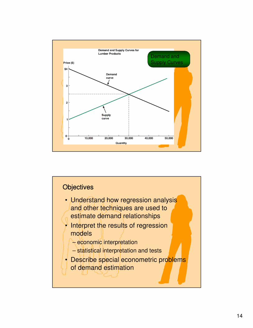
Demand and

Supply Curves

ObjectivesObjectives

• Understand how regression analysis

and other techniques are used to

estimate demand relationships

• Interpret the results of regression

models

– economic interpretation

– statistical interpretation and tests

• Describe special econometric problems

of demand estimation

15

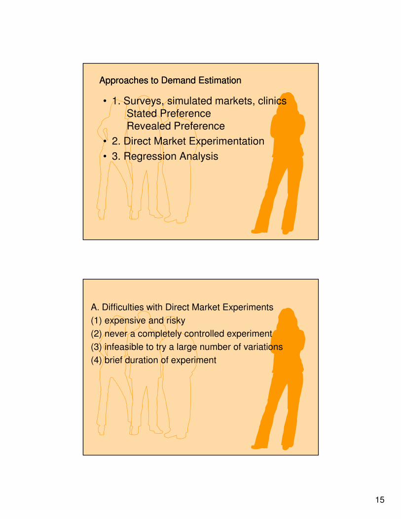
Approaches to Demand EstimationApproaches to Demand Estimation

• 1. Surveys, simulated markets, clinics

Stated Preference

Revealed Preference

• 2. Direct Market Experimentation

• 3. Regression Analysis

A. Difficulties with Direct Market Experiments

(1) expensive and risky

(2) never a completely controlled experiment

(3) infeasible to try a large number of variations

(4) brief duration of experiment

16

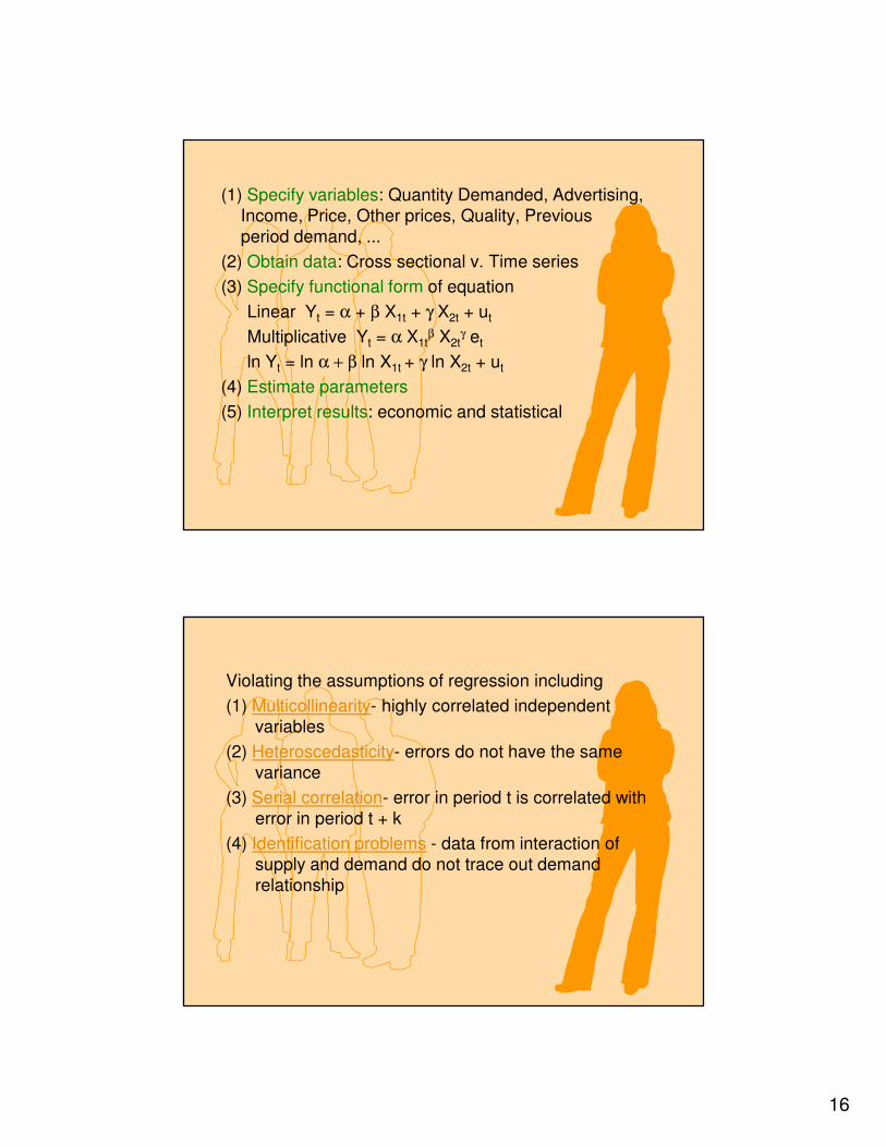
(1) Specify variables: Quantity Demanded, Advertising,

Income, Price, Other prices, Quality, Previous

period demand, ...

(2) Obtain data: Cross sectional v. Time series

(3) Specify functional form of equation

Linear Yt = α + β X1t + γ X2t + ut

Multiplicative Yt = α X1tβ X2t

γ et

ln Yt = ln α + β ln X1t + γ ln X2t + ut

(4) Estimate parameters

(5) Interpret results: economic and statistical

Violating the assumptions of regression including

(1) Multicollinearity- highly correlated independent

variables

(2) Heteroscedasticity- errors do not have the same

variance

(3) Serial correlation- error in period t is correlated with

error in period t + k

(4) Identification problems - data from interaction of

supply and demand do not trace out demand

relationship

17

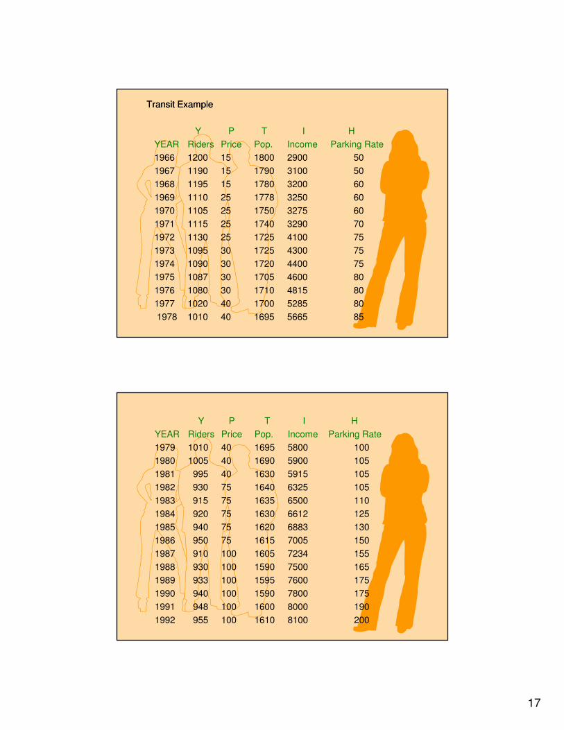
Transit ExampleTransit Example

Y P T I H

YEAR Riders Price Pop. Income Parking Rate

1966 1200 15 1800 2900 50

1967 1190 15 1790 3100 50

1968 1195 15 1780 3200 60

1969 1110 25 1778 3250 60

1970 1105 25 1750 3275 60

1971 1115 25 1740 3290 70

1972 1130 25 1725 4100 75

1973 1095 30 1725 4300 75

1974 1090 30 1720 4400 75

1975 1087 30 1705 4600 80

1976 1080 30 1710 4815 80

1977 1020 40 1700 5285 80

1978 1010 40 1695 5665 85

Y P T I H

YEAR Riders Price Pop. Income Parking Rate

1979 1010 40 1695 5800 100

1980 1005 40 1690 5900 105

1981 995 40 1630 5915 105

1982 930 75 1640 6325 105

1983 915 75 1635 6500 110

1984 920 75 1630 6612 125

1985 940 75 1620 6883 130

1986 950 75 1615 7005 150

1987 910 100 1605 7234 155

1988 930 100 1590 7500 165

1989 933 100 1595 7600 175

1990 940 100 1590 7800 175

1991 948 100 1600 8000 190

1992 955 100 1610 8100 200

18

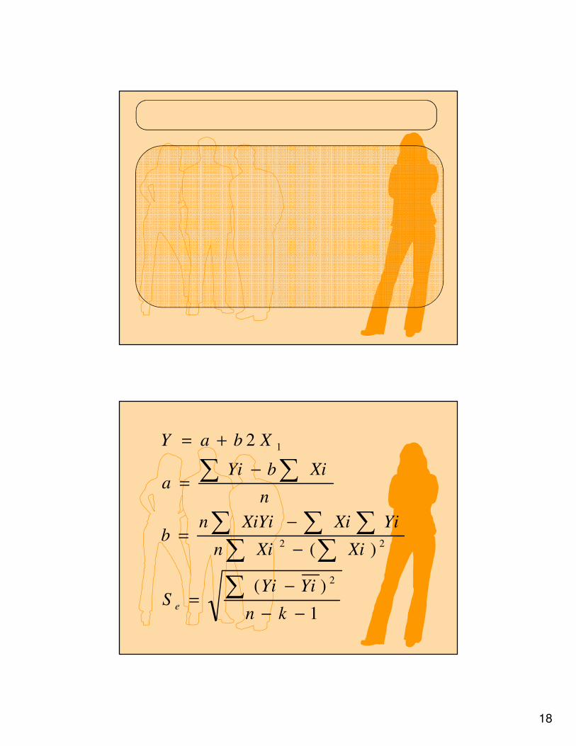
1

)(

)(

2

2

22

1

−−

−=

−

−=

−=

+=

∑

∑∑∑ ∑ ∑

∑ ∑

kn

YiYiS

XiXin

YiXiXiYinb

n

XibYia

XbaY

e

19

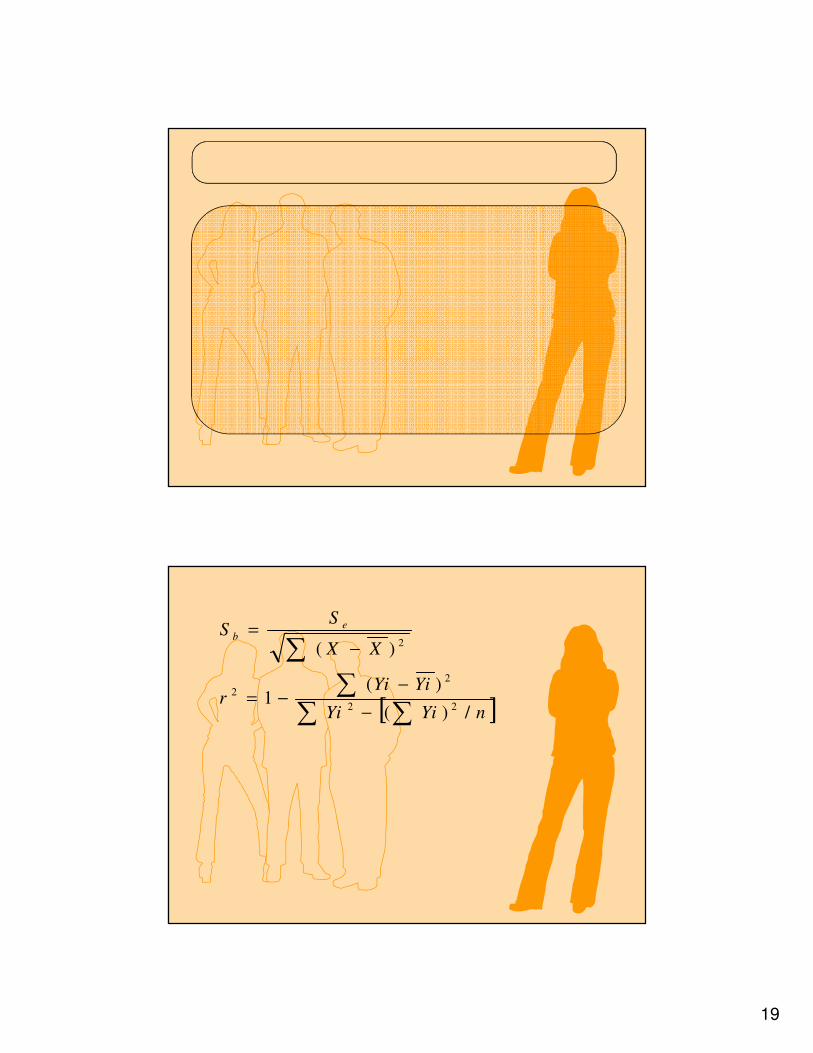
[ ]nYiYi

YiYir

XX

SS e

b

/)(

)(1

)(

22

2

2

2

∑∑∑

∑

−

−−=

−=

20

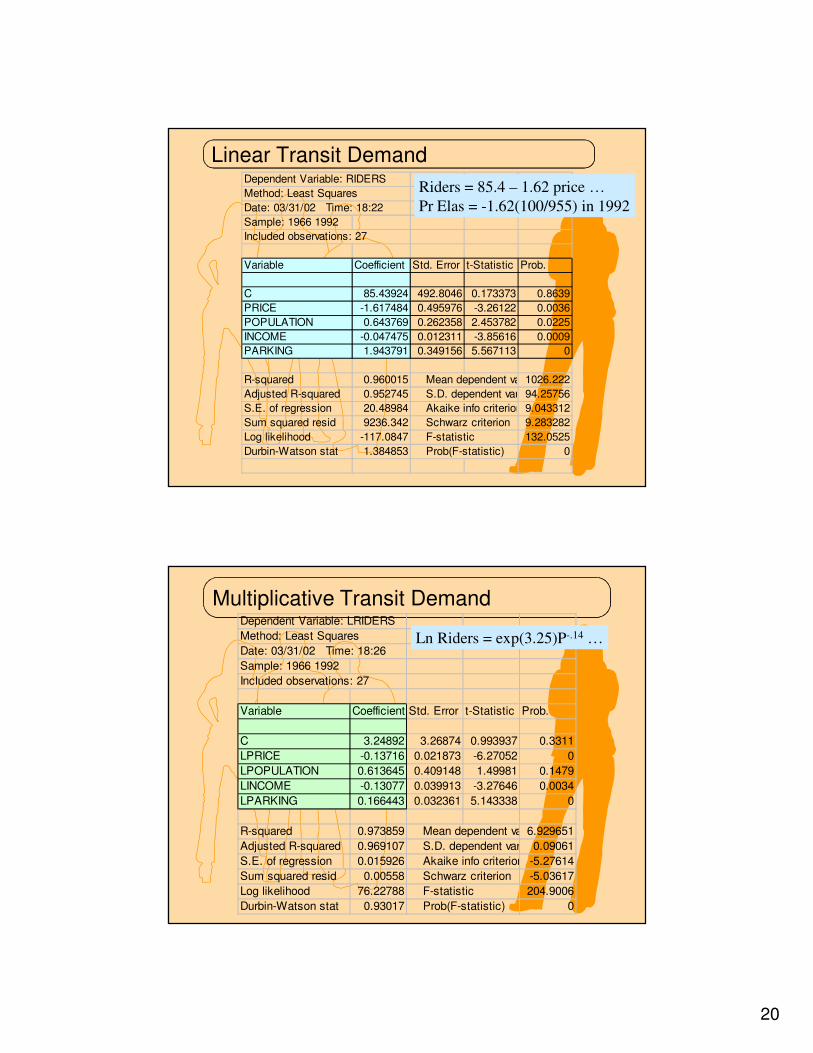
Linear Transit DemandDependent Variable: RIDERS

Method: Least Squares

Date: 03/31/02 Time: 18:22

Sample: 1966 1992

Included observations: 27

Variable Coefficient Std. Error t-Statistic Prob.

C 85.43924 492.8046 0.173373 0.8639

PRICE -1.617484 0.495976 -3.26122 0.0036

POPULATION 0.643769 0.262358 2.453782 0.0225

INCOME -0.047475 0.012311 -3.85616 0.0009

PARKING 1.943791 0.349156 5.567113 0

R-squared 0.960015 Mean dependent var1026.222

Adjusted R-squared 0.952745 S.D. dependent var 94.25756

S.E. of regression 20.48984 Akaike info criterion 9.043312

Sum squared resid 9236.342 Schwarz criterion 9.283282

Log likelihood -117.0847 F-statistic 132.0525

Durbin-Watson stat 1.384853 Prob(F-statistic) 0

Riders = 85.4 – 1.62 price …

Pr Elas = -1.62(100/955) in 1992

Multiplicative Transit DemandDependent Variable: LRIDERS

Method: Least Squares

Date: 03/31/02 Time: 18:26

Sample: 1966 1992

Included observations: 27

Variable Coefficient Std. Error t-Statistic Prob.

C 3.24892 3.26874 0.993937 0.3311

LPRICE -0.13716 0.021873 -6.27052 0

LPOPULATION 0.613645 0.409148 1.49981 0.1479

LINCOME -0.13077 0.039913 -3.27646 0.0034

LPARKING 0.166443 0.032361 5.143338 0

R-squared 0.973859 Mean dependent var6.929651

Adjusted R-squared 0.969107 S.D. dependent var 0.09061

S.E. of regression 0.015926 Akaike info criterion -5.27614

Sum squared resid 0.00558 Schwarz criterion -5.03617

Log likelihood 76.22788 F-statistic 204.9006

Durbin-Watson stat 0.93017 Prob(F-statistic) 0

Ln Riders = exp(3.25)P-.14 …

21

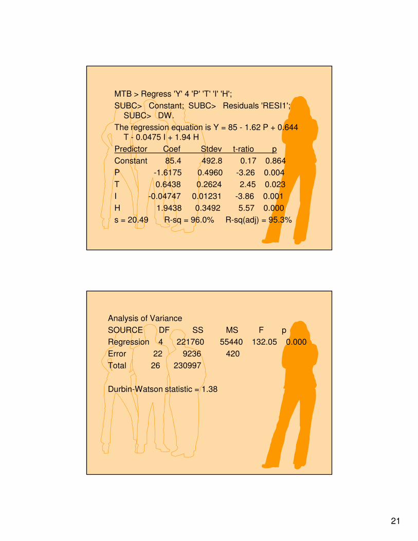
MTB > Regress 'Y' 4 'P' 'T' 'I' 'H';

SUBC> Constant; SUBC> Residuals 'RESI1';

SUBC> DW.

The regression equation is Y = 85 - 1.62 P + 0.644

T - 0.0475 I + 1.94 H

Predictor Coef Stdev t-ratio p

Constant 85.4 492.8 0.17 0.864

P -1.6175 0.4960 -3.26 0.004

T 0.6438 0.2624 2.45 0.023

I -0.04747 0.01231 -3.86 0.001

H 1.9438 0.3492 5.57 0.000

s = 20.49 R-sq = 96.0% R-sq(adj) = 95.3%

Analysis of Variance

SOURCE DF SS MS F p

Regression 4 221760 55440 132.05 0.000

Error 22 9236 420

Total 26 230997

Durbin-Watson statistic = 1.38

22

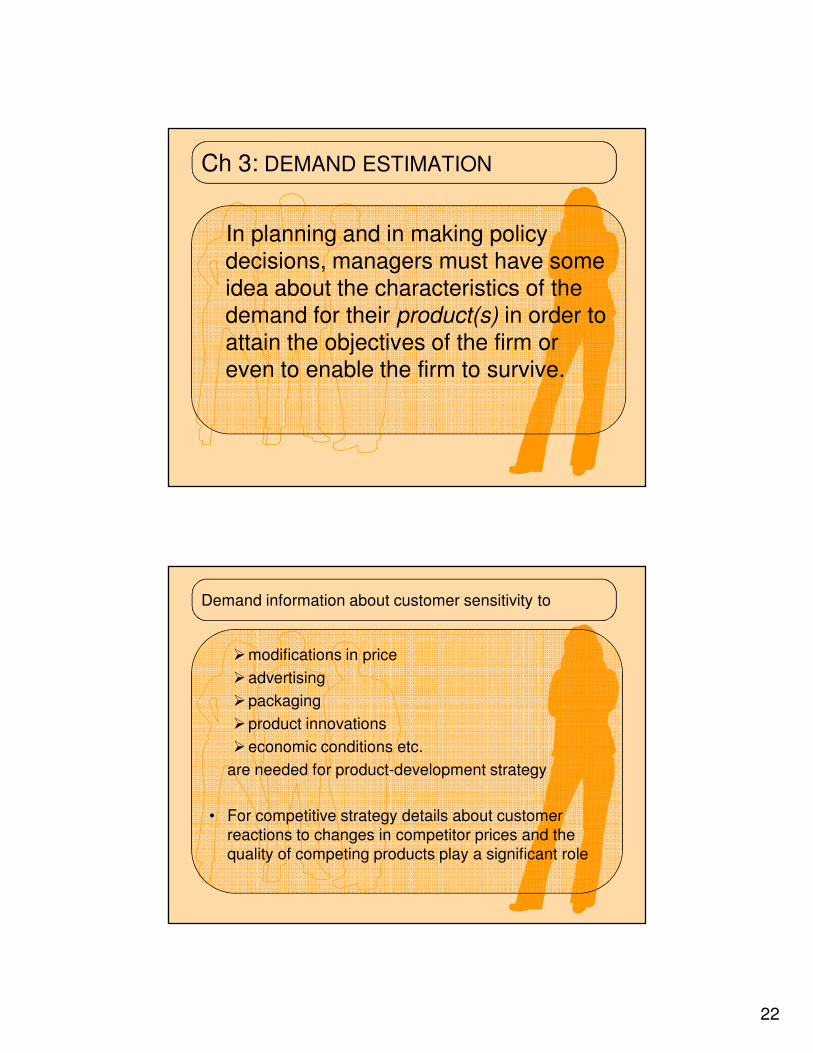
Ch 3: DEMAND ESTIMATION

In planning and in making policy decisions, managers must have some idea about the characteristics of the demand for their product(s) in order to attain the objectives of the firm or even to enable the firm to survive.

Demand information about customer sensitivity to

�modifications in price

�advertising

�packaging

�product innovations

�economic conditions etc.

are needed for product-development strategy

• For competitive strategy details about customer

reactions to changes in competitor prices and the

quality of competing products play a significant role

23

What Do Customers Want?

• How would you try to find out customer behavior?

• How can actual demand curves be estimated?

From Theory to Practice

D: Qx = f(px, Y, ps, pc, Τ, N)

(px=price of good x, Y=income, ps=price of substitute,

pc=price of complement, Τ=preferences, N=number

of consumers)

• What is the true quantitative relationship between

demand and the factors that affect it?

• How can demand functions be estimated?

• How can managers interpret and use these

estimations?

24

Most common methods used are:

a) consumer interviews or surveys

� to estimate the demand for new products

� to test customers reactions to changes in the price or advertising

� to test commitment for established products

b) market studies and experiments

� to test new or improved products in controlled settings

c) regression analysis

� uses historical data to estimate demand functions

Consumer Interviews (Surveys)

• Ask potential buyers how much of the

commodity they would buy at different

prices (or with alternative values for the

non-price determinants of demand)

�face to face approach

�telephone interviews

25

Consumer Interviews cont’d

• Problems:

– Selection of a representative sample

• what is a good sample?

– Response bias

• how truthful can they be?

– Inability or unwillingness of the

respondent to answer accurately

Market Studies and Experiments

• More expensive and difficult technique

for estimating demand and demand

elasticity is the controlled market study

or experiment

– Displaying the products in several different stores, generally in areas with different characteristics, over a period of time

• for instance, changing the price, holding

everything else constant

26

Market Studies and Experiments cont’d

• Experiments in laboratory or field

– a compromise between market studies and surveys

– volunteers are paid to stimulate buying conditions

Market Studies and Experiments cont’d

• Problems in conducting market studies and

experiments:

a) expensive

b) availability of subjects

c) do subjects relate to the problem, do they

take them seriously?

BUT: today information on market behavior also

collected by membership and award cards

27

Regression Analysis and Demand Estimation

• A frequently used statistical technique in demand estimation

• Estimates the quantitative relationship between the dependent variable and independent variable(s)

�quantity demanded being the dependent variable

� if only one independent variable (predictor) used: simple regression

� if several independent variables used: multiple regression

A Linear Regression Model

• In practice the dependence of one

variable on another might take any

number of forms, but an assumption of

linear dependency will often provide an

adequate approximation to the true

relationship

28

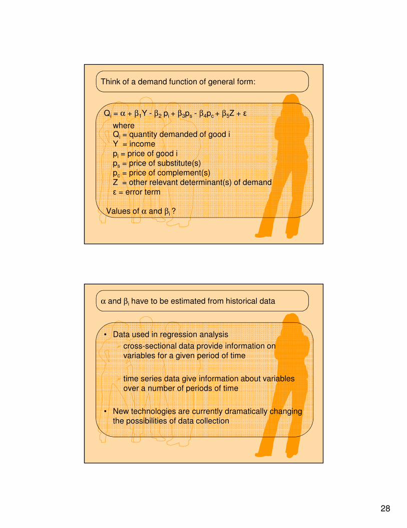
Think of a demand function of general form:

Qi = α + β1Y - β2 pi + β3ps - β4pc + β5Z + ε

whereQi = quantity demanded of good i

Y = income

pi = price of good i

ps = price of substitute(s)

pc = price of complement(s)

Z = other relevant determinant(s) of demand

ε = error term

Values of α and βi ?

α and βi have to be estimated from historical data

• Data used in regression analysis

�cross-sectional data provide information on

variables for a given period of time

� time series data give information about variables

over a number of periods of time

• New technologies are currently dramatically changing

the possibilities of data collection

29

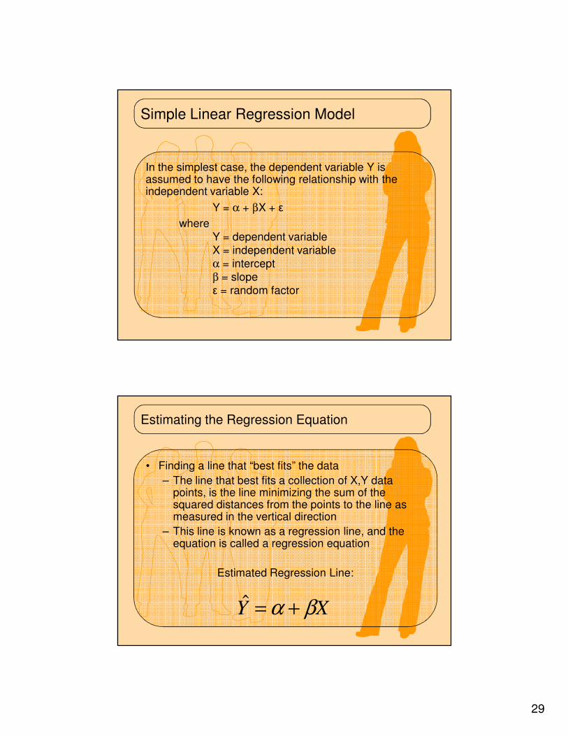
Simple Linear Regression Model

In the simplest case, the dependent variable Y is assumed to have the following relationship with the independent variable X:

Y = α + βX + ε

where

Y = dependent variable

X = independent variable

α = intercept

β = slope

ε = random factor

Estimating the Regression Equation

• Finding a line that “best fits” the data

– The line that best fits a collection of X,Y data points, is the line minimizing the sum of the squared distances from the points to the line as measured in the vertical direction

– This line is known as a regression line, and the equation is called a regression equation

Estimated Regression Line:

XY βα +=ˆ

30

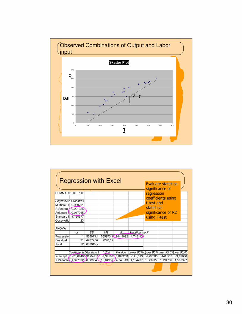
Observed Combinations of Output and Labor inputObserved Combinations of Output and Labor input

Skatter Plot

0

100

200

300

400

500

600

0 100 200 300 400 500 600 700 800

L

Q

Q

YY −ˆ

Regression with Excel

SUMMARY OUTPUT

Regression Statistics

Multiple R 0,959701

R Square 0,921026

Adjusted R Square0,917265

Standard Error47,64577

Observations 23

ANOVA

df SS MS F Significance F

Regression 1 555973,1 555973,1 244,9092 4,74E-13

Residual 21 47672,52 2270,12

Total 22 603645,7

CoefficientsStandard Errort Stat P-value Lower 95%Upper 95%Lower 95,0%Upper 95,0%

Intercept -75,6948 31,64911 -2,39169 0,026208 -141,513 -9,87686 -141,513 -9,87686

X Variable 11,377832 0,088043 15,64957 4,74E-13 1,194737 1,560927 1,194737 1,560927

Evaluate statistical significance of regression coefficients using t-test and statistical significance of R2 using F-test

31

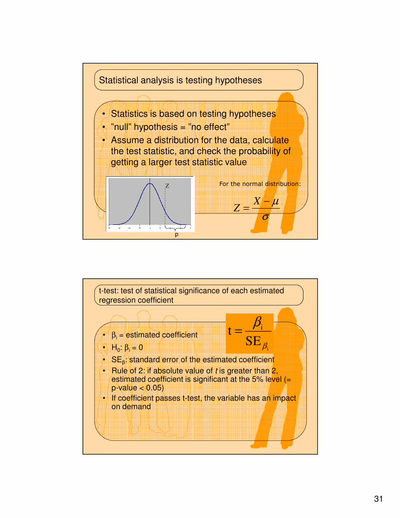
Statistical analysis is testing hypotheses

• Statistics is based on testing hypotheses

• ”null” hypothesis = ”no effect”

• Assume a distribution for the data, calculate the test statistic, and check the probability of getting a larger test statistic value

σ

µ−=

XZ

Z For the normal distribution:

p

t-test: test of statistical significance of each estimated

regression coefficient

• βi = estimated coefficient

• H0: βi = 0

• SEβ: standard error of the estimated coefficient

• Rule of 2: if absolute value of t is greater than 2, estimated coefficient is significant at the 5% level (= p-value < 0.05)

• If coefficient passes t-test, the variable has an impact on demand

iSE

t i

β

β=

32

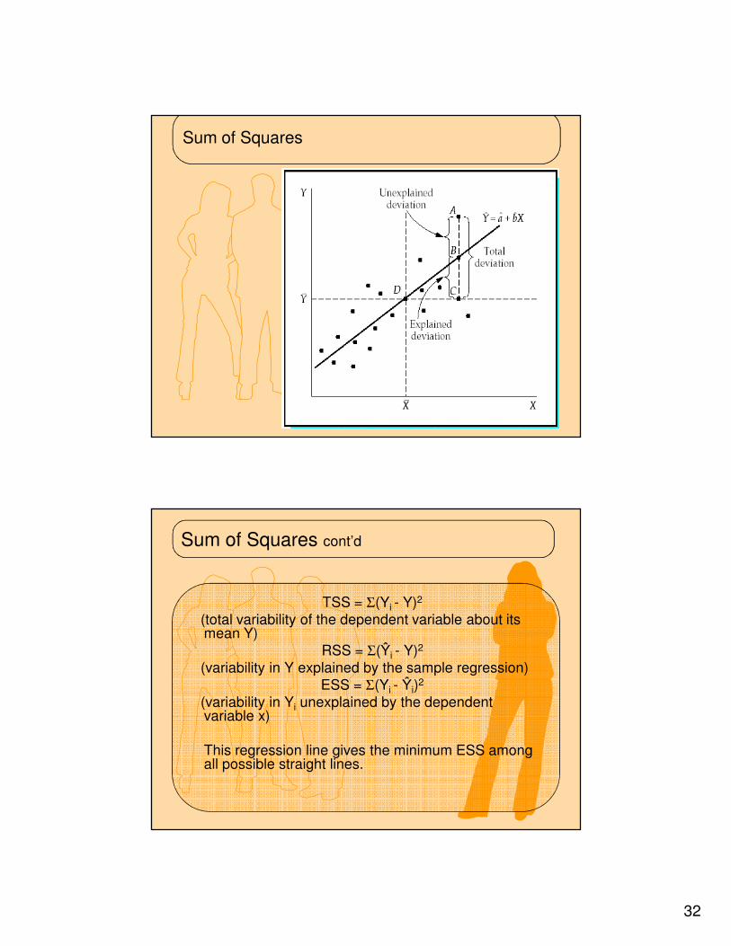
Sum of Squares

Sum of Squares cont’d

TSS = Σ(Yi - Y)2

(total variability of the dependent variable about its mean Y)

RSS = Σ(Ŷi - Y)2

(variability in Y explained by the sample regression)

ESS = Σ(Yi - Ŷi)2

(variability in Yi unexplained by the dependent variable x)

This regression line gives the minimum ESS among all possible straight lines.

33

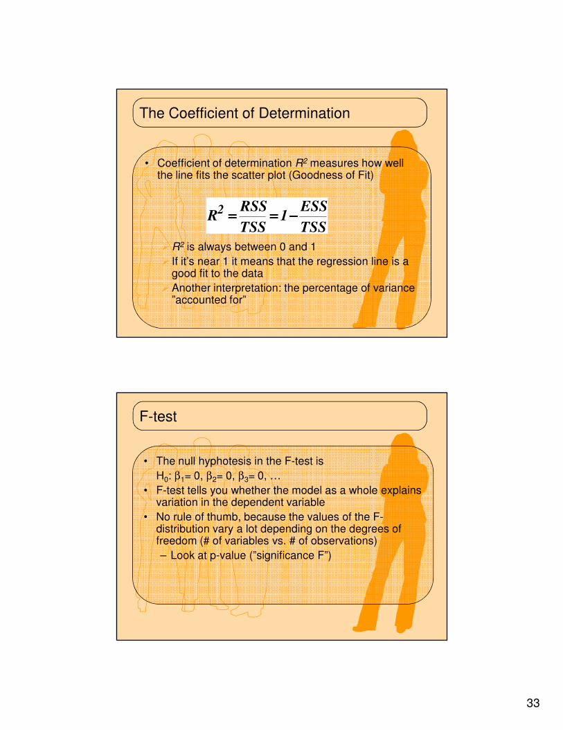
The Coefficient of Determination

• Coefficient of determination R2 measures how well the line fits the scatter plot (Goodness of Fit)

�R2 is always between 0 and 1

� If it’s near 1 it means that the regression line is a good fit to the data

�Another interpretation: the percentage of variance ”accounted for”

TSS

ESS1

TSS

RSSR

2 −−−−========

F-test

• The null hyphotesis in the F-test is

H0: β1= 0, β2= 0, β3= 0, …

• F-test tells you whether the model as a whole explains variation in the dependent variable

• No rule of thumb, because the values of the F-distribution vary a lot depending on the degrees of freedom (# of variables vs. # of observations)

– Look at p-value (”significance F”)

34

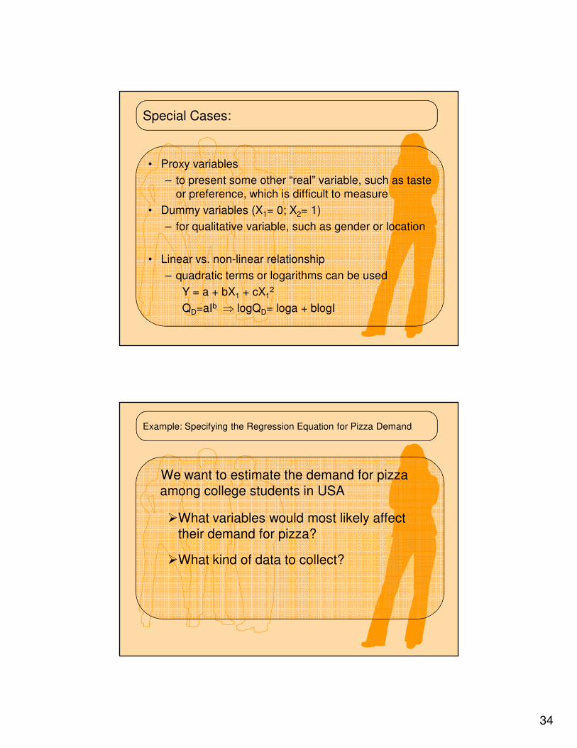
Special Cases:

• Proxy variables

– to present some other “real” variable, such as taste

or preference, which is difficult to measure

• Dummy variables (X1= 0; X2= 1)

– for qualitative variable, such as gender or location

• Linear vs. non-linear relationship

– quadratic terms or logarithms can be used

Y = a + bX1 + cX12

QD=aIb ⇒ logQD= loga + blogI

Example: Specifying the Regression Equation for Pizza Demand

We want to estimate the demand for pizza among college students in USA

�What variables would most likely affect their demand for pizza?

�What kind of data to collect?

35

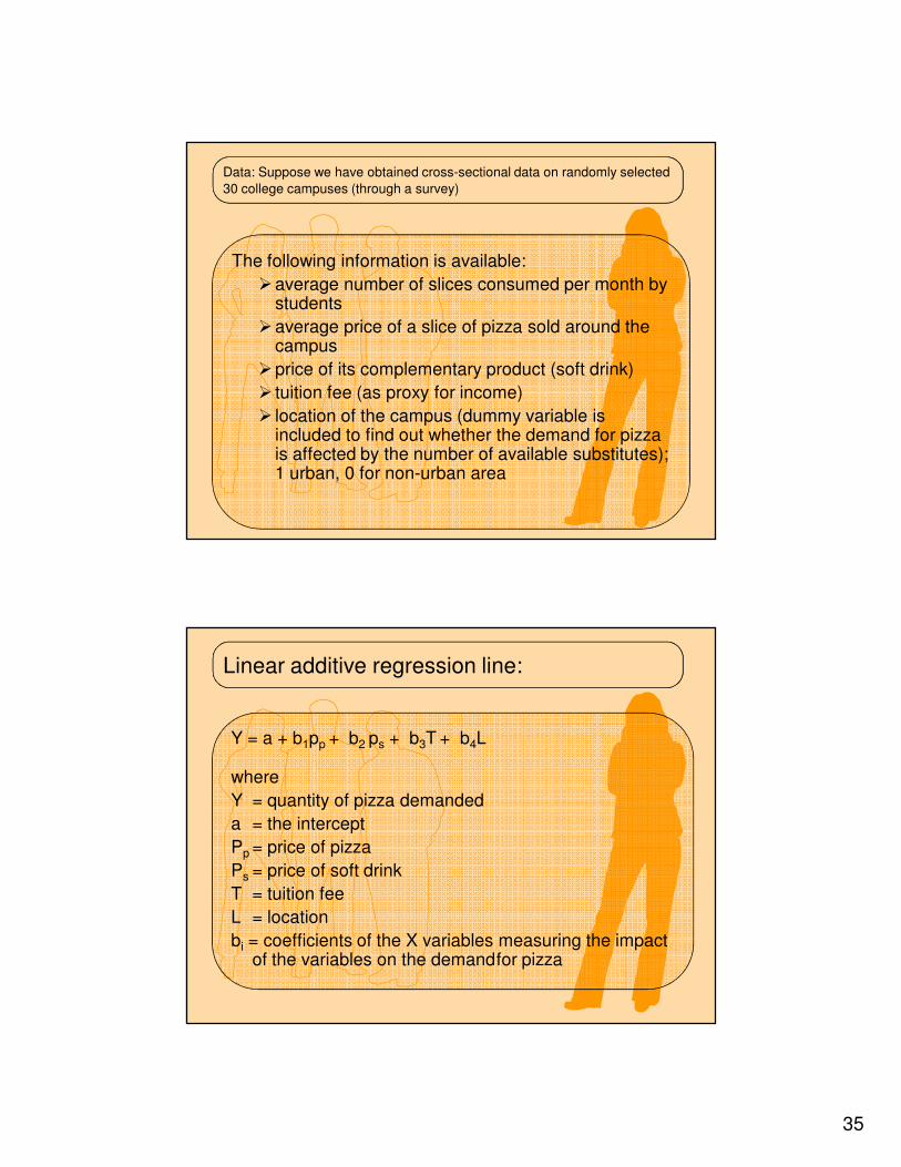
Data: Suppose we have obtained cross-sectional data on randomly selected

30 college campuses (through a survey)

The following information is available:

�average number of slices consumed per month by students

�average price of a slice of pizza sold around the campus

�price of its complementary product (soft drink)

� tuition fee (as proxy for income)

� location of the campus (dummy variable is included to find out whether the demand for pizza is affected by the number of available substitutes); 1 urban, 0 for non-urban area

Linear additive regression line:

Y = a + b1pp + b2 ps + b3T + b4L

where

Y = quantity of pizza demanded

a = the intercept

Pp = price of pizza

Ps = price of soft drink

T = tuition fee

L = location

bi = coefficients of the X variables measuring the impact of the variables on the demandfor pizza

36

Coefficients

Estimating and Interpreting the Regression

Coefficients

Y = 26.27- 0.088pp - 0.076ps + 0.138T- 0.544 L

(0.018) (0.018)* (0.020)* (0.087) (0.884)

R2 = 0.717

adjusted R2 = 0.67

F = 15.8

Numbers in parentheses are standard errors of coefficients.

*significant at the 0.01 level

Problems in the Use of Regression Analysis:

• identification problem

• multicollinearity

(correlation of coefficients)

• autocorrelation

(Durbin-Watson test)

• normality assumption fails

(outside the scope of this course)

37

Identification Problem

• Can arise when all effects on Y are not accounted for by

the predictors

Q

P

Q

P S

D3

D2

D1

Can demand be upward sloping?!

OR…?

D?!

Multicollinearity

• A significant problem in multiple

regression which occurs when there is a

very high correlation between some of

the predictor variables.

38

Resulting problem:

Regression coefficients may be very misleading or

meaningless because…

– their values are sensitive to small changes in the

data or to adding additional observations

– they may even be opposite in sign from what

”makes sense”

– their t-value (and the standard error) may change

a lot depending upon which other predictors are in

the model

Multicollinearity cont’d

Solution:

Don’t use two predictors which are very highly

correlated (however, x and x2 are O.K.)

Not a major problem if we are only trying to fit the data

and make predictions and we are not interested in

interpreting the numerical values of the individual

regression coefficients.

39

Multicollinearity cont’d

• One way to detect the presence of multicollinearity is to examine the correlation matrix of the predictor variables. If a pair of these have a high correlation they both should not be in the regression equation – delete one.

Y X1 X2 X3

Y 1.00 -.45 .81 .86

X1 -.45 1.00 -.82 -.59

X2 .81 -.82 1.00 .91

X3 .86 -.59 .91 1.00

Correlation Matrix

Autocorrelation

• Correlation between consecutive observations

• Usually encountered with time series data

– E.g. seasonal variation in demand

� Creates a problem with t-tests: insignificant variables may appear significant

time

D

40

A test for Autocorrelated Errors:DURBIN-WATSON TEST

• A statistical test for the presence of autocorrelation

• Fit the time series with a regression model and then

determine the residuals:

ttt yy ˆ−=ε

∑

∑

=

=

−−

=n

t

t

n

t

tt

d

1

2

2

2

1)(

ε

εε

The Interpretation of d:

The Durbin-Watson value d will always be

0 ≤ d ≤ 4

40 2

No correlation

Strong negative correlation

Strong positive correlation

41

Multiple Regression Procedure

1. Determine the appropriate predictors and the form of the regression model

– Linear relationship

– No multicollinearity

– Variables ”make sense”

2. Estimate the unknown α and β coefficients

3. Check the “goodness” of the model (R2, global F-test, individual t-test for each β coefficient)

4. Use the fitted model for predictions (and determine their accuracy)

Additional Comments:

• OCCAM’S RAZOR. We want a model that does a

good job of fitting the data using a minimum number

of predictors. A high R2 is not the only goal; variables

used should be ”meaningful”

• Don’t use more predictors in a regression model than

5% to 10% of n

• Correlation is not causality!

42

FORECASTING

• Expert opinion –based methods

– Delphi method

• Data-based methods

– Time series analysis

• History can predict the future?

– Regression analysis

• Forecast the values of the Xi’s to get Y

• Assumes the relationship between Xi’s and Y

does not change