INdica INTELLIGENT DECISION SUPPORT SYSTEM FOR … · Pertanian dan Asas Tani, MADA, MARDI, LPP dan...

VOT 74133

INdica- INTELLIGENT DECISION SUPPORT SYSTEM FOR RICE YIELD

PREDICTION IN PRECISION FARMING

INdica-SISTEM BANTUAN KEPUTUSAN PINTAR UNTUK RAMALAN PENGHASILAN PADI DALAM PRECISION FARMING

PUTEH BINTI SAAD ARYATI BAKRI

SITI SAKIRA KAMARUDIN MAHMAD NOR JAAFAR

FAKULTI SAINS KOMPUTER & SISTEM MAKLUMAT UNIVERSITI TEKNOLOGI MALAYSIA SEKOLAH TEKNOLOGI MAKLUMAT

UNIVERSITI UTARA MALAYSIA

i

ABSTRACT

Indica is an intelligent decision support system for rice yield prediction based on eleven (11) input parameters such as; weeds, rusiga, daun lebar, padi angin, bena perang, worms, rats,bacteria, jalur daun merah, hawar and lodging (kerebahan). The system is ported on a web server and is available freely on the internet. The outstanding feature of this system is the IDSS architecture that incorporates a neural network model as an intelligent component. The outstanding attributes of Indica are that; it is able to predict rice yield faster, easy to use and users can change input parameters easily. This system is useful for; Ministry of Agriculture & Agro-Based Industry, Malaysian Agriculture Development Association (MADA), Malaysian Agricultural Research and Development Institute (MARDI), Lembaga Pertubuhan Peladang (LPP) and private sectors. Ministry of Agriculture & Agro-Based Industry will use it in setting agricultural policy in national planning. MADA will use it to manage the efficiency of water usage in the rice field. MARDI will use it to support Research & Development activities especially in the area of precision farming. LPP will use it to offer advice to paddy farmers to produce improved quality rice with less damage to the environment and better utilization of water. In terms of sosio-economic impact, it will help farmers to produce high quantity of rice yield without jeopardizing the quality. It is anticipated that with the adoption of this system in the farmer’s farming practice will assure that the production of high quality rice will then be sufficient for local consumption as well as to be exported. Thus, per capita income of farmers will be increased.

ii

ABSTRAK

Indica merupakan sistem bantuan keputusan untuk meramal hasil padi berdasarkan sebelas (11) parameter input yang terdiri daripada; rumput rampai, rusiga, daun lebar, padi angin, bena perang, cacing, tikus,bakteria, jalur daun merah, hawar dan padi rebah. Sistem ini diletakkan di server sesawang yang boleh dicapai secara percuma melalui internet. Ciri yang menarik pada sistem ini ialah terdapatnya rangkaian neural selaku suatu komponen pintar yang disepadukan kedalam senibinanya. Sistem ini mampu meramal hasil padi dengan pantas, ianya mudah digunakan serta pengguna boleh menukar parameter input secara mudah. Sistem ini boleh digunakan oleh Kementerian Pertanian dan Asas Tani, MADA, MARDI, LPP dan sektor swasta. Kementerian Pertanian dan Asas Tani boleh menggunakannya untuk merangka polisi pertanian dalam perancangan nasional. Manakala pihak MADA boleh menggunakan sistem ini untuk mengurus penggunaan air secara efisien dikawasan penanaman padi. Pihak MARDI menggunakannya untuk menyokong aktiviti penyelidikan dan pembangunan dalam bidang ’precision farming’. Pihak LPP menggunakan sistem ini untuk membantu penanam padi menghasilkan beras yang bermutu tinggi tanpa merosakan persekitaran serta menggunakan air secara optimum. Adalah dijangkakan hasil pengeluaran padi akan meningkat dan ianya mencukupi untuk kegunaan negara dan juga boleh diekspot jika sistem ini digunakan dengan sepenuhnya. Oleh yang demikian pendapatan per capita penanam padi akan bertambah.

CONTENTS

CHAPTER CONTENT PAGE ABSTRACT

ABSTRAK

ACKNOWLEDGEMENT

1 INTRODUCTION

1.1 Background of the Problem 1 1.2 Statement of the Problem 2 1.3 Aim 3 1.4 Objective 3 1.5 Scope 4 1.6 Thesis Organization 4

2 LITERATURE REVIEW 6

2.1 Introduction 6 2.2 Precision Farming 7 2.3 ORYZA2000 9 2.4 Other crop yield modelling 10 2.5 Intelligent Decision Support System 12 2.6 Neural Network 16 2.6.1 Backpropagation Algorithm 17 2.6.2 Enhanced Backpropagation Algorithm 18 2.6.3 Radial Basis Function Network 19 2.7 Summary 20

3 RICE YIELD DATA AND DATA CONVERSION ALGORITHM

21

3.1 Introduction 21 3.2 Rice Yield Data 21 3.3 Data Conversion Algorithm 22 3.4 Summary 30

4 ARTIFICIAL NEURAL NETWORK MODEL 31 4.1 Introduction 31 4.2 Modeling the Rice Yield Data 32 4.3 ANN Parameters and Architecture 34 4.4 Performance of Conversion Algorithms using BP

ANN Model 35

4.5 Performance of Enhanced BP ANN Model 37 4.6 Performance of RBF ANN Model 41 4.7 Gradient Descent with Momentum and Adaptive

Learning Backpropagation 44

4.8 Summary 45

5 IDSS ARCHITECTURE AND PROTOTYPE 46 5.1 Introduction 46 5.2 IDSS Architecture 46 5.2.1 Predictive Model 47 5.2.2 Decision Support System 47 5.2.3 Web Development 48 5.2.4 Farming Database 49 5.2.5 User 50 5.3 IndiCA – the IDSS Prototype 50 5.4 Summary 55

6 CONCLUSION AND RECOMMENDATION 56 6.1 Conclusion 56 6.2 Recommendation 57 REFERENCES 58

iii

ACKNOWLEDGEMENT

Our deepest gratitude goes to Allah s.w.t. who gave us strength and endurance to

complete this research. We express our greatest gratitude to the Muda Agriculture

Development Authority (MADA) officers who provided the rice plantation data

collection for the purpose of this research. Without the data none of the work produced

in this research can be completed.

Grateful acknowledgment is made for research funding under the Intensified Research in

Priority Areas (IRPA) by the Ministry of Science, Technology and the Environment

(MOSTE) Malaysia, and the Faculty of Computer Science and Information System,

Universiti Teknologi Malaysia for providing the facilities to conduct the research. We

also express our sincere thanks to everyone, especially internal evaluators Assoc. Prof.

Daut Daman and external evaluators Prof Dr. Tengku Mohamad Tengku Sembok who

offered their idea and views during discussions and progress presentations on this

research. The project leader would like to offer sincere thanks to School of Computer &

Communication Engineering, KUKUM for providing the warm environment to pursue

this research.

We wish to thank our research officers; Nor Khairah Jamaludin, Noraslina Abdul

Rahman and S Niza Bajuri and research assistants; Khairul Azhan, Shahrul Nizam

Yaakob and Muhammad Firdaus Hashim for helpful effort in making this project a

success. We also thank our colleagues for their time and assistance at various stages

during the development of this report and the research that led up to it. Finally, our

warmest appreciation goes to our family, this research would not have been possible

without their support, inspiration, encouragement co-operation and prayers.

LIST OF TABLES

Table Title

Page

3.1 List of Input Parameters 22 3.2 A Sample of Raw Data for Musim 1/1995 obtained from

MADA 23

3.3 Results Using Principal Component Analysis 24 3.4 Normalization Techniques 25 3.5 Results of Using Techniques A (Simple Normalization) 3.6 Results of Using Techniques B (Improved Simple

Normalization) 27

3.7 Results of Using Techniques C (Unit Range) 28 3.8 Results of Using Techniques D (Improved Unit Range) 29 3.9 Results of Using Techniques E (Improved Linear

Scaling) 30

4.1 Neural Network Parameters 35 4.2 Mean Deviation During Training 37 4.3 Number of Nodes in the Hidden Layer for the Learning

Algorithms 39

4.4 Sum Squared Error and Number of Neurons 43 4.5 Mean Square error and epochs 43

LIST OF FIGURES

FIGURE NUMBER TITLE PAGE 2.0 The decision-

Making/Modelling process 14

2.1 Unified architecture for an intelligent decision support system

15

4.1 Modelling steps using the ANN model

33

4.2 Back propagation ANN Model

34

4.3 Normalization techniques vs. Mean deviation during training

36

4.4 Mean deviation vs. Normalization Techniques during prediction

37

4.5 Average Absolute Error versus Different Enhanced back propagation Alghorithms

40

4.6 Yield versus Locality of quick propagation

41

4.7 Yield versus Locality of Conjugate Gradient Descent

41

4.8 Yield versus Locality of Levenberg-Marquardt

41

4.9 Yield versus Locality of Back Propagation

41

4.10 Sum squared error of the RBF network plotted against number of neurons

43

4.11 Mean squared error of the MLP network plotted against its epochs

44

5.1 Architecture of the IDSS for rice Yield Prediction

48

5.2 Web-based development of IDSS for rice Yield prediction

49

5.3 Main page of IndiCA-the IDSS prototype

51

5.4 IndiCA1 interface A 52 5.5 IndiCA1 interface A 53 5.6 Pest Management Interface

A 54

5.7 Pest Management Interface B

55

CHAPTER 1

INTRODUCTION

1.1 Background of the Problem

Precision farming is a new method of crop management by which areas of land or

crop within a field may be managed by different levels of input depending upon the

yield potential of the crop in that particular area of land. Precision farming is an

integrated agricultural management system incorporating several technologies such

as global positioning system, geographical information system, yield monitor and

variable rate technology [1]. Precision farming has the potential to reduce costs

through more efficient and effective applications of crop inputs and it can also reduce

environmental impacts by allowing farmers to apply inputs only where they are

needed at the appropriate rate [2].

Meanwhile, prediction can be considered as one of the oldest crop management

activities [3]. Prediction of crops yield like wheat, corn and rice has always been an

interesting research area to agro meteorologist and it has become an important

economic concern [4]. Rice is the world’s most important food crop and a primary

source of food for more than half of the world’s population [5]. Almost 90% of rice

is produced and consumed in Asia, and 96% in developing countries [6]. In

Malaysia, The Third Agriculture Policy (1998-2010) was established to meet at least

70% of Malaysia’s demand a 5% increase over the targeted 65%. The remaining

30% comes from imported rice mainly from Thailand, Vietnam and China [7].

2

Raising level of national rice self-sufficiency has become a strategic issue in the

agricultural ministry of Malaysia. The numerous problem associated with rise

farming include monitoring the status of nutrient soil, maintaining irrigation

infrastructures, obtaining quality seedlings, controlling pests, weeds and diseases,

and many other problems that need to be addressed in order to increase productivity

[8]. All these problems can be overcome with a good prediction system which can

foresee rice yield in the near future.

The ability to predict the future enables the farm managers to take the most

appropriate decision in anticipation of that future. Neural network offers exciting

possibilities to perform machine learning and prediction, and abundantly utilized in

performing agriculture prediction task [4][9][10][11]. Safa et. al, 2002 used

Backpropagation Network to predict wheat yield using climatic observation data and

predicted with a maximum of 45-60kg/ha. Sudduth et. al, 1996 used neural network

to predict soy bean yield based on soil parameters and achieve a testing error of

17.3%. Liu et. al, 2001 used NN to predict maize yield based on rainfall, soil and

other parameters and obtained a testing error of 14.8%, whereas O’Neal et. al, 2002

used Backpropagation Network to predict rice yield based on weather data

[4][9][11]. Neural network has the ability to learn and identify complex patterns of

information and to associate input data and output.

1.2 Statement of the Problem

In this study we intend to come up with an approach of developing IDSS for rice

yield prediction in precision farming. The research question is:

How to produce an approach that is able to predict rice yield based on real input

parameters collected from MUDA Irrigation areas?

3

In order to answer the main issue raised above, the following issues need to be

addressed as a pre-requisite:

a. What is the suitable technique to perform the data conversion processes?

b. What is the suitable Neural Network Model to be used as the intelligent

component in the IDSS?

c. What is the suitable architecture for the IDSS?

d. How to develop the IDSS prototype?

e. What is the suitable platform to place the IDSS prototype so that the

interested parties/organization able to access it globally?

1.3 Aim

The goal of this project is to develop an intelligent decision support system that can

predict rice yield based on specified input parameters.

1.4 Objective

The objectives of this project are:

(a) To identify the format and values for input parameters affecting

the rice yield

(b) To investigate, design and develop data conversion and reduction

algorithm for input parameters affecting rice yield.

4

(c) To study relevant Artificial Neural Network (ANN) Models and

propose a suitable ANN Model as an intelligent component in the

IDSS.

(d) To propose the architecture to predict crop yield given the input

parameters.

(e) To design and develop an intelligent decision support system for rice

yield prediction.

1.5 Scope

The scope of this study is as follows:

(a) There are eleven (11) input parameters being considered namely;

weeds, rusiga, daun lebar, padi angin, bena perang, worms,

rats,bacteria, jalur daun merah, hawar and lodging

(b) Data were obtained from the Muda Irrigation Area, Alor Star, Kedah

Muda Agricultural Development Authority (MADA) ranges from

1995 to 2001, a total of seven (7) years.

1.6 Thesis Organization

The report consists of six (6) chapters. Each chapter is briefly described as

follows:

(a) Chapter 1 describes the background of the problem, statement of the

problem, aim, objective, scope and ended with report organization.

5

(b) Chapter 2 contains a definition of precision farming, a review on the

existing crop modeling system, a description of an intelligent decision

support system and the ANN Model.

(c) Chapter 3 presents the yield data obtained from MADA and

illustrations of various data conversion algorithms.

(d) Chapter 4 describes the evaluated ANN Models and a proposed

model.

(e) Chapter 5 describes the Intelligent Decision Support System (IDSS)

architecture and the IDSS prototype.

(f) Chapter 6 presents the Conclusion and Recommendations.

6

CHAPTER 2

LITERATURE REVIEW

2.1 Introduction

Before the 1980’s, the agriculture sector was considered an important income earner for

most Malaysians. Nevertheless, Malaysia is currently competing among other global

players in other new emerging businesses, technologies and industries such as the

automobile sector, telecommunication and biotechnology industry. However, this

country has never undermine the importance of the nation’s first and foremost bread

winner for the country; agriculture. Even after the 2004 General Election, the

importance and well being of the agriculture industry has been reinforced. Previously,

all pertaining issues and activities regarding agriculture, livestock, farming, fishery and

commodities were totally under the Ministry of Agriculture. A new milestone in the

agriculture sector has been proven due to the establishment of a new ministry solely for

the interest of this sector, the Ministry of Agriculture and Agro-Based Industry.

Currently, this ministry is responsible for improving the income of farmers, livestock

breeders and fisherman by efficient utilization of the nation’s resources. Additional it

also helps to manage food production for the domestic consumption and export [20].

Since the mid-60s, raising the level of national rice self-sufficiency and the income of

paddy farming households has been a strategic political issue in Malaysia. One of the

7

approaches in obtaining the maximum quantity of rice yield is by using precision

farming. It is a comprehensive system designed to optimize agriculture production by

carefully tailoring soil and crop management to fit the different conditions found in each

field while maintaining environmental quality. The advantages of precision farming is

that it offers opportunities to improve agriculture productivity and product quality,

reduces agro-chemical wastage through efficient application and resulting in minimizing

environmental pollution and in energy conservation[1][2].

Thus this chapter starts with a definition of precision farming concept, then a review on

the existing crop modeling system, a description of an intelligent decision support

system and the ANN Model.

2.2 Precision Farming

Precision farming is a new agricultural system concept with the goals of optimizing

returns in agricultural production and environment. Today’s technological advancement

has reached a level where a farmer can have access to information and tools to manage

mechanized in-field operations. They can now measure, evaluate and deal with in-field

variability, (e.g. soil fertility, water availability and yield) that was known to exist

previously but was not manageable, to his advantage. The ability to handle variations in

productivity within a field and maximize financial return, reduce waste and minimize

impact on the environment has always been the objective of an enterprising farmer,

especially those with limited land resources and those who advocate sound agriculture

practice.

This concept is not new. What is new is the ability to automate data collection and

documentation and the utilization of this information for strategic farm management

decision in the field operations through mechanization, sensing and communication

technology. To some, precision farming means using satellite, sensors and field or

thematic maps. Precision farming is in fact a comprehensive system designed to

8

optimize agriculture production by carefully tailoring soil and crop management to fit

the different conditions found in each field while maintaining environmental quality

[1][2]. Current whole-field management approaches ignore variability in soil-related

characteristics and seek to apply crop production inputs in a uniform manner. With such

approach there was obviously the likelihood of over-application and under-application

of inputs in a single field. The advantages of precision farming is it offers opportunities

to improve agriculture productivity and product quality, reduces agro-chemical wastage

through efficient application and resulting in minimizing environmental pollution and in

energy conservation. In precision farming timeliness of in-field operations (cultivation,

seed sowing, application of fertilizers and pesticides and harvest) is crucial. Precision

farming has, therefore, not only the ability to apply treatments that are varied at local

level, but also to precisely monitor and assess the agricultural enterprise at a local and

farm level. It also provides sufficient understanding of the processes involved to apply

inputs in such a way as to be able to achieve a particular goal. The goal, however, might

not necessarily mean maximum yield but may be to optimize financial advantage while

operating within environmental constraints.

In-field variability, spatially or temporally, in soil-related properties, crop

characteristics, weed and insect population and harvest data are important database that

need to be developed to realize the potential of precision farming. Of these, entire crop

yield monitoring, is the most mature component of precision farming technology and is

the logical starting point for precision farming. It gives the farmer something to look at

and start raising question about his management. Several years of yield data may be

required to make good decision. Highly varying yield within a field indicate that the

current management practices may not be providing the best possible growing

conditions everywhere in the field. In this case, further adoption of precision farming for

the other operations may be beneficial.

Establishment of soil-related characteristics within a field, through regular soil sampling,

is another database that is extremely important. Some of the characteristics such as soil

texture vary very little with time, others such as moisture content, nitrate level, fluctuate

9

rapidly. Decision therefore has to be made on what property to sample, how to sample

and how often to sample so that interpretation from database can be made with greater

confidence. These soil variables can be very large and complex and is difficult to

manage and interpret. Therefore, it is critical to define the minimum data sets that

influence crop growth and production. More do not necessarily mean higher yield or

income but will surely increase cost through cost of analysis of the parameters

considered.

2.3 ORYZA2000

ORYZA2000 is an upgraded system for a SERE model of rice growth that was

developed in 1990 under simulation and system analysis for rice production. It is an

upgrading and integration between ORYZA1 (for potential production) and ORYZA-N

(for nitrogen-defender product). ORYZA 2000 simulates the growth and the

development of lowland rice at potential production situation, water limitation and

nitrogen limitation. To simulate situations of production, several module need to be

integrated in ORYZA2000. The aforementioned modules are; cropping module, evapo-

transpiration model, dynamic nitrogen module and water-soil balancing module. The

modules are coded in FORTRAN programming language to simulate agro ecological

growth process. Daily weather is used as the input data to the module.

ORYZA2000 simulate water-balance and cropping growth and also the growth of

lowland rice under potential and situation of water decrease and also the decreasing of

nitrogen. Under this condition, the model has been tested in field experiments using

variety of high modern result at tropical (such as IR20, IR58, IR64 and IR72 at IRRI in

Philippine) and sub-tropical (such as YRL39 at Yanco, Australia). Validity result had

been reported that is a potential production by Kropff et al (1994a,b) and Matthew et al

10

(1995), for production and water decrease by Wopereis (1993), Wopereis et al (1996a,b)

and Boling et al (2000), for production that the nitrogen decrease by Drenth et al (1994)

and Aggarwal et al [21]. For crop parameters, ORYZA2000 controlled the parameters

like pests and weeds and also the element of water and nitrogen. In all the experiments,

the crop is supplied with enough phosphorus and sodium. The rice field had been

protected from pests and weeds. In that situation, ORYZA2000 is expected to be

performed successfully for others type of paddy and also in other situation.

ORYZA2000 has not been tested on hybrid rice or other type of highland rice since

these types of rice requires more parameters.

2.4 Other crop yield modelling

Besides ORYZA2000, there are several crops system such as wheat, corn and grains. In

the wheat yield prediction, the researchers also apply artificial neural network by using

climatic data to predict dry farming wheat yield. In this study, the result of climatology

for period (1990-99) for each of eleven phenological stages as parameters of wheat

including germination, emergence, third leaves, tillerng, stem formation, heading,

flowering, milk maturity, wax maturity, full maturity and also meteorological factors.

Because of the purpose of this study is to predict wheat yield, the input vector elements

must be selected by factors affecting it. The most important of these elements are

meteorological factors such as: air temperature, wind speed, rainfall quantity, interval

rainfall, sun hours, air relative humidity and evapotranspiration. The effect of radiation

factors (SSR, TSR, RSR) are considered as important parameters too. But, due to lack of

correct and complete statistic, it was not included in the input matrix. The wheat yield

was predicted with maximum error (45-60 kg/ha) at least two month before crop

ripening.

11

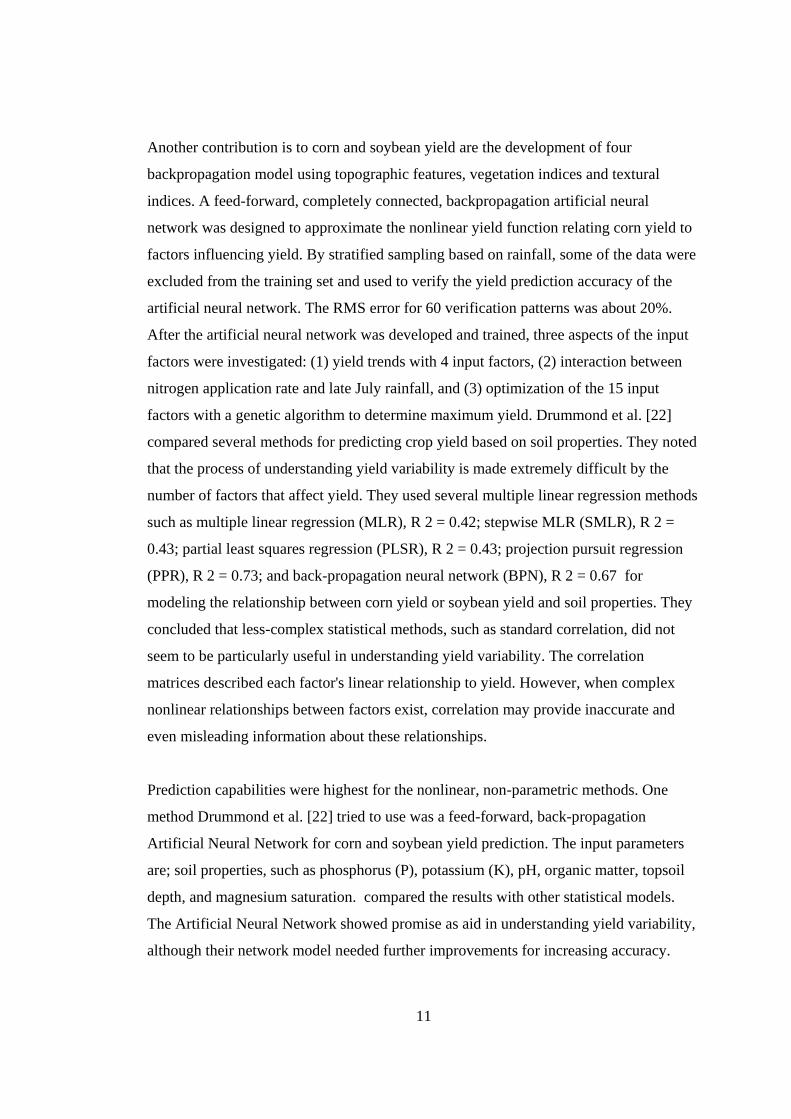
Another contribution is to corn and soybean yield are the development of four

backpropagation model using topographic features, vegetation indices and textural

indices. A feed-forward, completely connected, backpropagation artificial neural

network was designed to approximate the nonlinear yield function relating corn yield to

factors influencing yield. By stratified sampling based on rainfall, some of the data were

excluded from the training set and used to verify the yield prediction accuracy of the

artificial neural network. The RMS error for 60 verification patterns was about 20%.

After the artificial neural network was developed and trained, three aspects of the input

factors were investigated: (1) yield trends with 4 input factors, (2) interaction between

nitrogen application rate and late July rainfall, and (3) optimization of the 15 input

factors with a genetic algorithm to determine maximum yield. Drummond et al. [22]

compared several methods for predicting crop yield based on soil properties. They noted

that the process of understanding yield variability is made extremely difficult by the

number of factors that affect yield. They used several multiple linear regression methods

such as multiple linear regression (MLR), R 2 = 0.42; stepwise MLR (SMLR), R 2 =

0.43; partial least squares regression (PLSR), R 2 = 0.43; projection pursuit regression

(PPR), R 2 = 0.73; and back-propagation neural network (BPN), R 2 = 0.67 for

modeling the relationship between corn yield or soybean yield and soil properties. They

concluded that less-complex statistical methods, such as standard correlation, did not

seem to be particularly useful in understanding yield variability. The correlation

matrices described each factor's linear relationship to yield. However, when complex

nonlinear relationships between factors exist, correlation may provide inaccurate and

even misleading information about these relationships.

Prediction capabilities were highest for the nonlinear, non-parametric methods. One

method Drummond et al. [22] tried to use was a feed-forward, back-propagation

Artificial Neural Network for corn and soybean yield prediction. The input parameters

are; soil properties, such as phosphorus (P), potassium (K), pH, organic matter, topsoil

depth, and magnesium saturation. compared the results with other statistical models.

The Artificial Neural Network showed promise as aid in understanding yield variability,

although their network model needed further improvements for increasing accuracy.

12

They did not include weather information and other factors in their artificial neural

network.

An Artificial Neural Network trained to relate crop yield to the factors that affect yield

could be very useful in setting more realistic target yields within fields for precision

agriculture. Crop yields are highly dependent upon weather, which cannot be predicted.

However, all inputs except weather could be specified for a trained artificial neural

network. Many years of past weather records could then be input to calculate yield

variation with weather. From such calculations, it would be possible to calculate

probabilities of achieving crop yields at various levels. In selecting target yields, a

producer would then be able to estimate the probabilities of achieving those yields.

An artificial neural network trained to predict yield accurately in one field might not be

accurate in another field. If some unmeasured factors influenced yields, the training

process might set weights that compensated for the omissions in the field used for

training. If the level of those unmeasured factors differed in another field, the neural

network trained in the first field would be inaccurate in the second field. However, an

advantage of the Artificial Neural Network is that it may be practical to do initial

training on a field with a large database, and then retrain the network for other fields

with much smaller databases. The network topology could be the same for all fields, but

through retraining, the weights could be specific to each field. Moreover, the weights for

each field could be updated through retraining each time a new crop was harvested.

2.5 Intelligent Decision Support System

The first concepts involved in DSS were first articulated in the early 1970s by Scott-

Morton under the term management decision systems. He defined such system as

13

“Interactive compute-based systems, which can help decision makers, utilize data

and models to solve unstructured problems” [1971]. Another classical definition

of DSS, provided by Keen and Scott-Morton [1978] follows:

When the organization has complex decision to make or problem to solve, it often turns

to experts for advice. These experts have specific knowledge and experience in the

problem area. In other to make the system can solve the complex problem and get the

better decision the decision support system had to add with intelligent component so

that this component can handle the problem.

Adding the intelligence to the process of modeling (building models or using existing

models) and to their management makes lots of sense because some of the tasks

involved (e.g., modeling and selecting models) require considerable expertise. The

topics of intelligent modeling and intelligent model management have attracted

significant academic attention in recent years [12] because the potential benefits could

be substantial. It seems, however, that implement of such integration is fairly difficult

and slow.

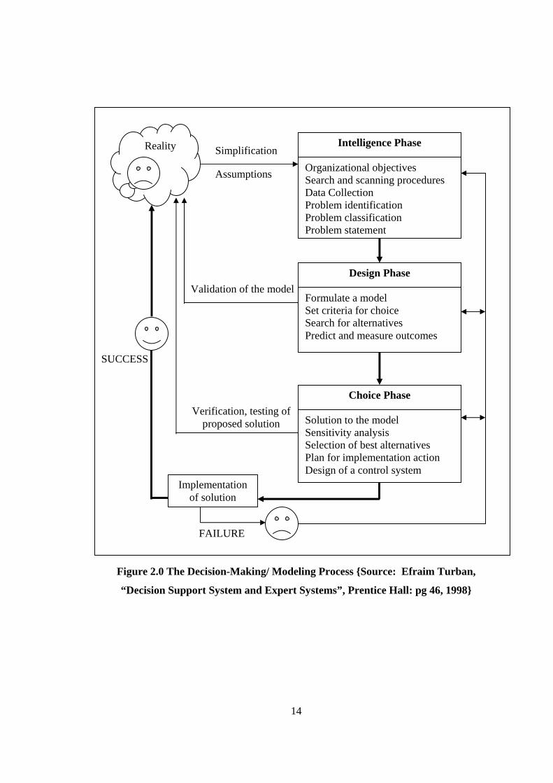
To better understand in modeling the decision-making process, it is advisable to follow

step according to Simon [1977], involve three major phases: intelligence, design and

choice. A fourth phase, implementation, was added later. A conceptual picture of the

decision-making process is shown in Figure 2.0. There is a continuous flow activities

from intelligent to design to choice, but at any phase there may be a return to a previous

phase.

The decision-making process starts with intelligent phase, where reality is examined and

the problem is identified and defined. In the design phase a model that represents the

system is constructed. This is done by making assumptions that simplify reality and by

writing the relationships among all variables. The courses actions are identified. The

choice phase includes a proposed solution of the model.

14

Figure 2.0 The Decision-Making/ Modeling Process {Source: Efraim Turban,

“Decision Support System and Expert Systems”, Prentice Hall: pg 46, 1998}

SUCCESS

Intelligence Phase

Organizational objectives Search and scanning procedures Data Collection Problem identification Problem classification Problem statement

Design Phase

Formulate a model Set criteria for choice Search for alternatives Predict and measure outcomes

Choice Phase

Solution to the model Sensitivity analysis Selection of best alternatives Plan for implementation action Design of a control system

Reality

Implementation of solution

Simplification

Assumptions

Validation of the model

Verification, testing of proposed solution

FAILURE

15

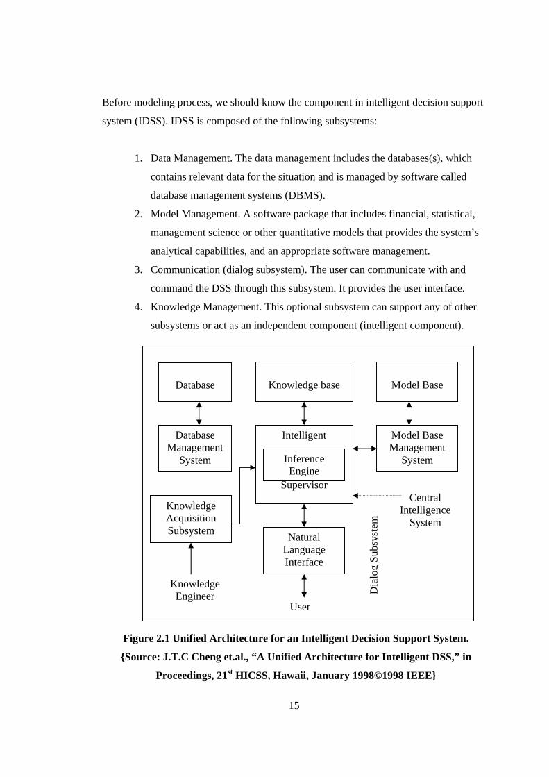
Before modeling process, we should know the component in intelligent decision support

system (IDSS). IDSS is composed of the following subsystems:

1. Data Management. The data management includes the databases(s), which

contains relevant data for the situation and is managed by software called

database management systems (DBMS).

2. Model Management. A software package that includes financial, statistical,

management science or other quantitative models that provides the system’s

analytical capabilities, and an appropriate software management.

3. Communication (dialog subsystem). The user can communicate with and

command the DSS through this subsystem. It provides the user interface.

4. Knowledge Management. This optional subsystem can support any of other

subsystems or act as an independent component (intelligent component).

Database

Knowledge base

Model Base

Database Management

System

Model Base Management

System

Intelligent

Supervisor

Inference Engine

Knowledge Acquisition Subsystem Natural

Language Interface

Central Intelligence

System

Knowledge Engineer

User

Dia

log

Subs

yste

m

Figure 2.1 Unified Architecture for an Intelligent Decision Support System.

{Source: J.T.C Cheng et.al., “A Unified Architecture for Intelligent DSS,” in

Proceedings, 21st HICSS, Hawaii, January 1998©1998 IEEE}

16

2.6 Neural Network

Neural network or more precisely, Artificial Neural Network (ANN) is also referred in

the literature as connectionist network or parallel-distributed processor [23]. It consists

of a large number of processing elements called neurons or nodes or units. These

processing elements are interconnected to each other and the power of neural network

lies in the tremendous number of interconnections and its learning capability. Neural

network can be defined as a massively parallel distributed processor that has a natural

propensity for storing experiential knowledge and making it available for used. The

motivation for the development of neural network technology stemmed from the desire

to develop an artificial system that could perform “intelligent” tasks similar to those

performed by human brain. Neural Networks have grown rapidly over the last few years, show good capability to

deal with non-linear multivariate systems. Moreover, they can process input patterns

never presented before, in much the same way as the human brain does. Recently,

connections have emerged between neural network techniques and its applications in

engineering, agricultural, and environmental sciences.

An artificial neural network is a computational mechanism that is able to acquire,

represent, and compute a weighting or mapping from one multivariate space of

information to another, given a set of data represent on that mapping. It can identify

subtle patterns in input training data which may be missed by conventional statistical

analysis. In contrast to regression models, neural networks do not require knowledge of

the functional relationships between the input and the output variables. Moreover, these

techniques are non-linear, and therefore may handle very complex data patterns which

make simulation modeling unattainable. As well as the ability to model multi-output

phenomena, another advantage of neural networks is that all kinds of data - continuous,

near-continuous, and categorical or binary - can be input without violating model

assumptions. Once the training and testing phases of the neural network analysis are

found to be successful, the generated algorithm can be easily put to use in practical

applications [24].

17

2.6.1 Backpropagation Algorithm

Backpropagation is most widely used learning algorithm. It is a popular technique

because it is easy to implement. It does require training data for conditioning the

network before using it for predicting the output. A backpropagation network includes

one or more hidden layers. The network is considered a feedforward approach, since

there are no interconnections between the output of a processing element and the input

of node on the same layer or on the preceding layer. Externally provided correct patterns

are compared with the neural network output during training (i.e., it is a supervised

training), and feedback is used to adjust the weights until all training patterns are

correctly categorized by the network.

Starting with the output layer, error between the actual and desired outputs is used to

correct the weights for the connections the previous layer. It has been shown that for any

output neuron, j, the error (delta) = (Zj – Yj) x (df/dx), where Z and Y are the actual

outputs. It is useful to choose the sigmoid function, f = [1 + exp (-x)]-1, to represent the

output of that neuron. In this way, df/dx = f (1 - f) and the error is a simple function of

the desired and actual outputs. The factor f (1 - f) is the logistic function, which serve to

keep the error correction well bounded. The weights of each input to the jth neuron are

then changed in proportion to this calculated error. A more complicated expression can

be derived to work backwards a similar way from the output neurons through the inner

layers to calculate the correction to the associated weights of the inner neurons.

Backpropagation algorithm has successfully used in predicted corn yield based on soil

texture, topography, Ph and some nutrient element [11]. Another application of

backpropagation algorithm is to predict wheat yield using climatic observation data [12].

18

2.6.2 Enhanced Backpropagation Algorithm Quick propagation computes the average gradient of the error surface across all cases

before updating the weights once at the end of the epoch.

In the standard BP, the error function decreases most rapidly along the negative of the

gradient however fastest convergence is not guaranteed. Conjugate gradient descent

overcomes the discrepancy by constructing a series of line searches across the error

surface. It first works out the direction of steepest descent, just as back propagation

would do [10][11].

00 gp −=

A line search is then performed to determine the optimal distance to move along the

current search direction

kkkk pxx α+=+1

where

xk is the vector of current weight and bias

αk is the learning rate

pk is the gradient

The next search direction is determined so that it is conjugate to previous search

directions. The general procedure for determining the new search direction is to

combine the new steepest descent direction with the previous search direction:

1−+−= kkkk pgp β

The constant βk is computed based on the Fletcher-Reeves update:

11 −−

=k

Tk

kTk

k gggg

β

19

The Levenberg-Marquardt algorithm was designed to approach second-order training

speed without having to compute the Hessian matrix. When the performance function

has the form of a sum of squares, then the Hessian matrix can be approximated as:[6][3]. H = JT J

and the gradient can be computed as

g = JT e

where

J : Jacobian matrix contains first derivatives of the network errors with respect

to the weights and biases.

E : a vector of network errors

The weights and biases are computed based on the following formula: [ ] eJIJJxx TT

kk1

1−

+ +−= µ where µ is a scalar value. µ is decreased after each successful step and is increased only when a tentative step

would increase the performance function. Hence, the performance function will always

be reduced at each iteration of the algorithm.

2.6.3 Radial Basis Function Network

Radial Basis Function (RBF) neural networks is an alternative to the popular Multi

Layer Perceptron (MLP) based neural networks that is used in conjunction with back

propogation training method for the generation neural network model. RBF neural

networks are function approximation models that can be trained by examples to

implement a desired input-output mapping [14]. Under most circumstances, the

performance of RBF neural networks can match those of back-propogation MLP.

20

RBF networks differs from MLP networks from a number of characteristics [15] MLP

based networks depends on the number of units per layer, RBF based networks requires

that the number of radial basis functions use centres and widths of those functions be

calculated earlier. RBF networks employs only one hidden layer and MLP networks may

have more than one hidden layer.

Nodes in MLP networks typically share a common neural model whereas hidden and

output nodes in RBF networks are functionally distinct. Another significant difference is

that MLP networks construct “global” approximations to non-linear output

approximations whereas RBF networks construct “local” input-output approximations

(Gaussian functions)[15].RBF network is created by adding a neuron to the hidden layer

one at a time until the (SSE) in formula reach below the value objective target.

2.7 Summary

This chapter contains a definition of precision farming, an evaluation of rice growth and

production simulation model, ORYZA2000. Besides ORYZA2000, other crop yield

models are also reviewed. The chapter then continues to describe an intelligent decision

support system (IDSS) methodology and architecture that will be adopted to predict the

rice yield. Artificial Neural Network (ANN) model will be used as the intelligent

component in the IDSS. Thus this chapter finally describes various ANN models that

are potentially to be chosen to predict rice yield, starting with Backpropagation Neural

Network Model, Enhanced Backpropagation Neural Network Model and Radial Basis

Function Network.

Next chapter contains examples of rice yield data and various data conversion

algorithms explored.

CHAPTER 3

RICE YIELD DATA AND CONVERSION ALGORITHMS

3.1 Introduction

In this chapter, processes to perform the first and second objectives of the project are

reported. To recap, the first objective is to identify the format and values for input

parameters affecting the rice yield. The second objective is to investigate, design and

develop data conversion and reduction algorithm for input parameters affecting rice

yield. Section 3.2 presents the rice yield data and Section 3.3 describes the data

conversion algorithms examined in this project.

3.2 Rice Yield Data

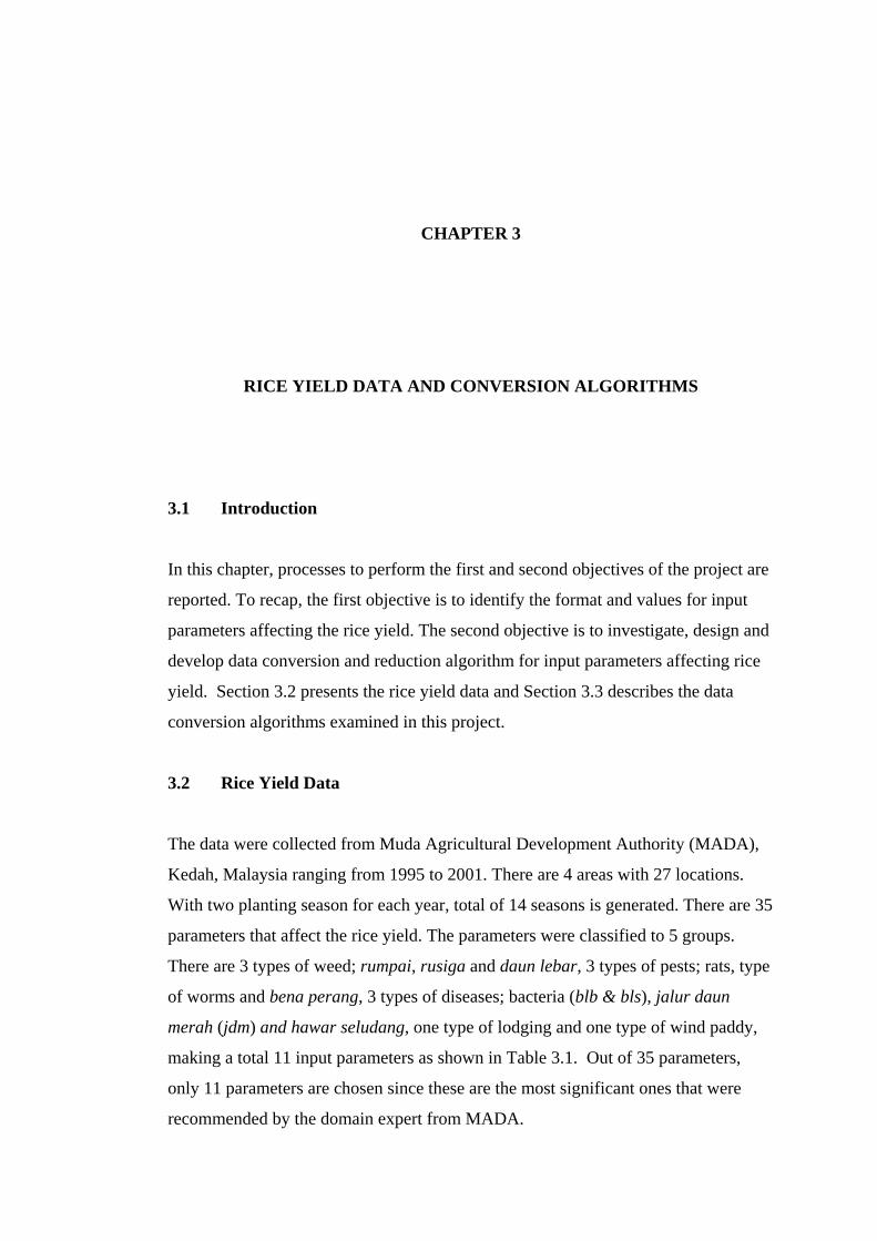
The data were collected from Muda Agricultural Development Authority (MADA),

Kedah, Malaysia ranging from 1995 to 2001. There are 4 areas with 27 locations.

With two planting season for each year, total of 14 seasons is generated. There are 35

parameters that affect the rice yield. The parameters were classified to 5 groups.

There are 3 types of weed; rumpai, rusiga and daun lebar, 3 types of pests; rats, type

of worms and bena perang, 3 types of diseases; bacteria (blb & bls), jalur daun

merah (jdm) and hawar seludang, one type of lodging and one type of wind paddy,

making a total 11 input parameters as shown in Table 3.1. Out of 35 parameters,

only 11 parameters are chosen since these are the most significant ones that were

recommended by the domain expert from MADA.

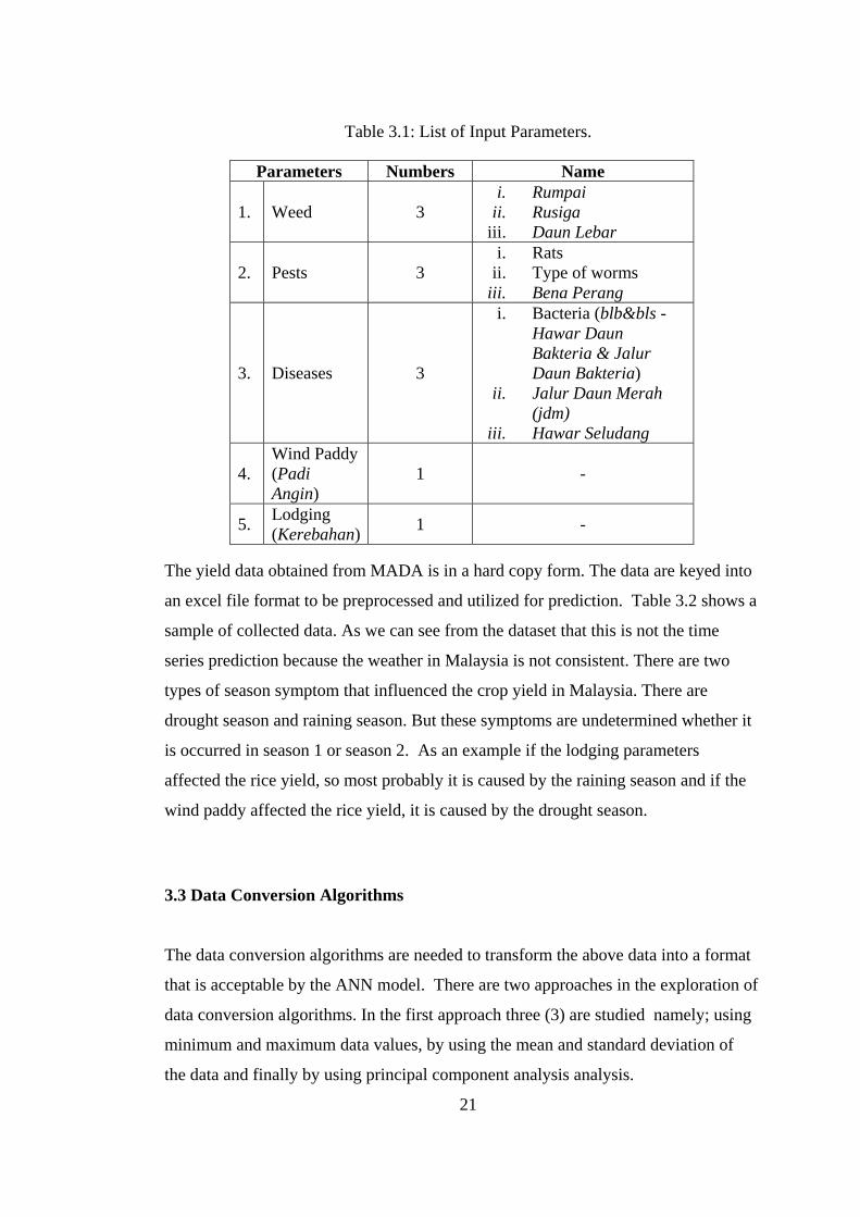
Table 3.1: List of Input Parameters.

The yield data obtained from MADA is in a hard copy form. The data are keyed into

an excel file format to be preprocessed and utilized for prediction. Table 3.2 shows a

sample of collected data. As we can see from the dataset that this is not the time

series prediction because the weather in Malaysia is not consistent. There are two

types of season symptom that influenced the crop yield in Malaysia. There are

drought season and raining season. But these symptoms are undetermined whether it

is occurred in season 1 or season 2. As an example if the lodging parameters

affected the rice yield, so most probably it is caused by the raining season and if the

wind paddy affected the rice yield, it is caused by the drought season.

3.3 Data Conversion Algorithms The data conversion algorithms are needed to transform the above data into a format

that is acceptable by the ANN model. There are two approaches in the exploration of

data conversion algorithms. In the first approach three (3) are studied namely; using

minimum and maximum data values, by using the mean and standard deviation of

the data and finally by using principal component analysis analysis.

21

Parameters Numbers Name

1. Weed 3 i. Rumpai

ii. Rusiga iii. Daun Lebar

2. Pests 3 i. Rats

ii. Type of worms iii. Bena Perang

3. Diseases 3

i. Bacteria (blb&bls - Hawar Daun Bakteria & Jalur Daun Bakteria)

ii. Jalur Daun Merah (jdm)

iii. Hawar Seludang

4. Wind Paddy (Padi Angin)

1 -

5. Lodging (Kerebahan) 1 -

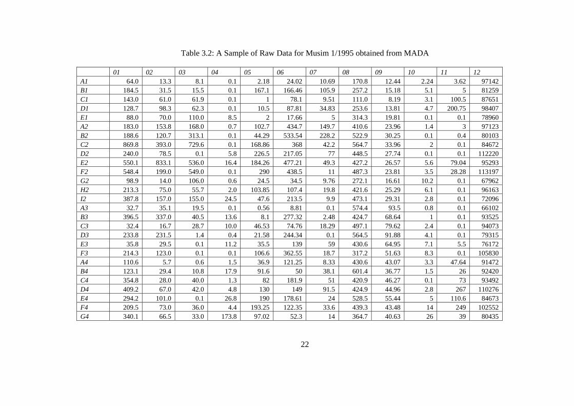
Table 3.2: A Sample of Raw Data for Musim 1/1995 obtained from MADA

01 02 03 04 05 06 07 08 09 10 11 12 A1 64.0 13.3 8.1 0.1 2.18 24.02 10.69 170.8 12.44 2.24 3.62 97142 B1 184.5 31.5 15.5 0.1 167.1 166.46 105.9 257.2 15.18 5.1 5 81259 C1 143.0 61.0 61.9 0.1 1 78.1 9.51 111.0 8.19 3.1 100.5 87651 D1 128.7 98.3 62.3 0.1 10.5 87.81 34.83 253.6 13.81 4.7 200.75 98407 E1 88.0 70.0 110.0 8.5 2 17.66 5 314.3 19.81 0.1 0.1 78960 A2 183.0 153.8 168.0 0.7 102.7 434.7 149.7 410.6 23.96 1.4 3 97123 B2 188.6 120.7 313.1 0.1 44.29 533.54 228.2 522.9 30.25 0.1 0.4 80103 C2 869.8 393.0 729.6 0.1 168.86 368 42.2 564.7 33.96 2 0.1 84672 D2 240.0 78.5 0.1 5.8 226.5 217.05 77 448.5 27.74 0.1 0.1 112220 E2 550.1 833.1 536.0 16.4 184.26 477.21 49.3 427.2 26.57 5.6 79.04 95293 F2 548.4 199.0 549.0 0.1 290 438.5 11 487.3 23.81 3.5 28.28 113197 G2 98.9 14.0 106.0 0.6 24.5 34.5 9.76 272.1 16.61 10.2 0.1 67962 H2 213.3 75.0 55.7 2.0 103.85 107.4 19.8 421.6 25.29 6.1 0.1 96163 I2 387.8 157.0 155.0 24.5 47.6 213.5 9.9 473.1 29.31 2.8 0.1 72096 A3 32.7 35.1 19.5 0.1 0.56 8.81 0.1 574.4 93.5 0.8 0.1 66102 B3 396.5 337.0 40.5 13.6 8.1 277.32 2.48 424.7 68.64 1 0.1 93525 C3 32.4 16.7 28.7 10.0 46.53 74.76 18.29 497.1 79.62 2.4 0.1 94073 D3 233.8 231.5 1.4 0.4 21.58 244.34 0.1 564.5 91.88 4.1 0.1 79315 E3 35.8 29.5 0.1 11.2 35.5 139 59 430.6 64.95 7.1 5.5 76172 F3 214.3 123.0 0.1 0.1 106.6 362.55 18.7 317.2 51.63 8.3 0.1 105830 A4 110.6 5.7 0.6 1.5 36.9 121.25 8.33 430.6 43.07 3.3 47.64 91472 B4 123.1 29.4 10.8 17.9 91.6 50 38.1 601.4 36.77 1.5 26 92420 C4 354.8 28.0 40.0 1.3 82 181.9 51 420.9 46.27 0.1 73 93492 D4 409.2 67.0 42.0 4.8 130 149 91.5 424.9 44.96 2.8 267 110276 E4 294.2 101.0 0.1 26.8 190 178.61 24 528.5 55.44 5 110.6 84673 F4 209.5 73.0 36.0 4.4 193.25 122.35 33.6 439.3 43.48 14 249 102552 G4 340.1 66.5 33.0 173.8 97.02 52.3 14 364.7 40.63 26 39 80435

22

where

01 jenis rumput 07 tikus 02 jenis rusiga 08 blb&bls (hawar daun

bakteria&jalur daun bakteria) 03 jenis daun lebar 09 jdm (jalur daun merah) 04 padi angin 10 hawar 05 bena perang 11 rebah 06 jenis ulat 12 hasil (output)

An to Gn represent locations

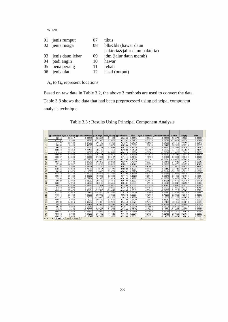
Based on raw data in Table 3.2, the above 3 methods are used to convert the data.

Table 3.3 shows the data that had been preprocessed using principal component

analysis technique.

Table 3.3 : Results Using Principal Component Analysis

23

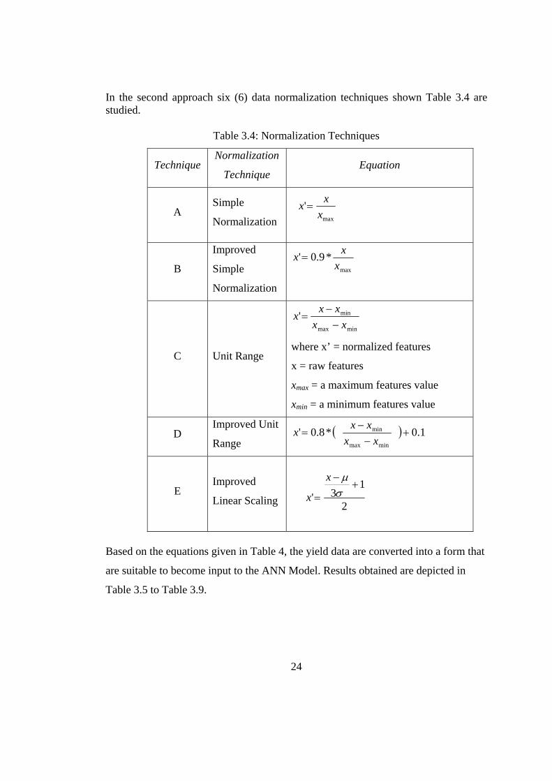
In the second approach six (6) data normalization techniques shown Table 3.4 are studied.

Table 3.4: Normalization Techniques

Technique Normalization

Technique Equation

A Simple

Normalization

B

Improved

Simple

Normalization

max

*9.0'x

xx =

C Unit Range

minmax

min'xx

xxx−

−=

where x’ = normalized features

x = raw features

xmax = a maximum features value

xmin = a minimum features value

D Improved Unit

Range ( ) 1.0*8.0'

minmax

min +−

−=

xxxxx

E Improved

Linear Scaling

Based on the equations given in Table 4, the yield data are converted into a form that

are suitable to become input to the ANN Model. Results obtained are depicted in

Table 3.5 to Table 3.9.

24

max

'x

xx =

2

13'

+−

= σµx

x

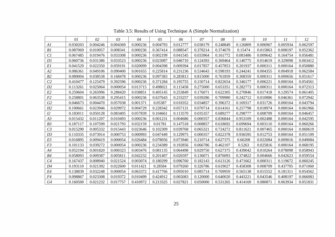
Table 3.5: Results of Using Technique A (Simple Normalization) 01 02 03 04 05 06 07 08 09 10 11 12

A1 0.030203 0.004246 0.004369 0.000236 0.004793 0.012777 0.038179 0.248849 0.126809 0.006967 0.005934 0.062597 B1 0.087069 0.010057 0.008341 0.000236 0.367414 0.088547 0.378214 0.374679 0.15474 0.015863 0.008197 0.052362 C1 0.067485 0.019476 0.033308 0.000236 0.002199 0.041545 0.033964 0.161772 0.083486 0.009642 0.164754 0.056481 D1 0.060736 0.031386 0.033523 0.000236 0.023087 0.046710 0.124393 0.369464 0.140775 0.014619 0.329098 0.063412 E1 0.041529 0.022350 0.059191 0.020099 0.004398 0.009394 0.017857 0.457853 0.201937 0.000311 0.000164 0.050880 A2 0.086361 0.049106 0.090400 0.001655 0.225814 0.231236 0.534643 0.598193 0.244241 0.004355 0.004918 0.062584 B2 0.089004 0.038538 0.168478 0.000236 0.097383 0.283813 0.815000 0.761859 0.308359 0.000311 0.000656 0.051617 C2 0.410477 0.125479 0.392596 0.000236 0.371284 0.195755 0.150714 0.822654 0.346177 0.006221 0.000164 0.054561 D2 0.113261 0.025064 0.000054 0.013715 0.498021 0.115458 0.275000 0.653351 0.282773 0.000311 0.000164 0.072313 E2 0.259604 0.265996 0.288420 0.038851 0.405145 0.253849 0.176071 0.622305 0.270846 0.017418 0.129574 0.061405 F2 0.258801 0.063538 0.295415 0.000236 0.637643 0.233257 0.039286 0.709980 0.242712 0.010886 0.046361 0.072942 G2 0.046673 0.004470 0.057038 0.001371 0.05387 0.018352 0.034857 0.396372 0.169317 0.031726 0.000164 0.043794 H2 0.100661 0.023946 0.029972 0.004729 0.228342 0.057131 0.070714 0.614161 0.257798 0.018974 0.000164 0.061966 I2 0.183011 0.050128 0.083405 0.057839 0.104661 0.113570 0.035357 0.689277 0.298777 0.008709 0.000164 0.046457 A3 0.015432 0.011207 0.010493 0.000236 0.001231 0.004686 0.000357 0.836844 0.953109 0.002488 0.000164 0.042595 B3 0.187117 0.107599 0.021793 0.032159 0.01781 0.147518 0.008857 0.618692 0.699694 0.003110 0.000164 0.060266 C3 0.015290 0.005332 0.015443 0.023646 0.102309 0.039768 0.065321 0.724272 0.811621 0.007465 0.000164 0.060619 D3 0.110335 0.073914 0.000753 0.000993 0.047449 0.129975 0.000357 0.822378 0.936595 0.012753 0.000164 0.051109 E3 0.016895 0.009419 0.000054 0.026484 0.078056 0.073940 0.210714 0.627375 0.66208 0.022084 0.009016 0.049084 F3 0.101133 0.039272 0.000054 0.000236 0.234389 0.192856 0.066786 0.462107 0.5263 0.025816 0.000164 0.068195 A4 0.052194 0.001820 0.000323 0.003476 0.081135 0.064498 0.029750 0.627375 0.439042 0.010264 0.078098 0.058943 B4 0.058093 0.009387 0.005811 0.042232 0.201407 0.026597 0.136071 0.876093 0.374822 0.004666 0.042623 0.059554 C4 0.167437 0.008940 0.021524 0.003074 0.180299 0.096760 0.182143 0.613126 0.471662 0.000311 0.119672 0.060245 D4 0.193110 0.021392 0.022600 0.011421 0.28584 0.079260 0.326786 0.619027 0.458308 0.008709 0.437705 0.071060 E4 0.138839 0.032248 0.000054 0.063372 0.417766 0.095010 0.085714 0.769959 0.565138 0.015552 0.181311 0.054562 F4 0.098867 0.023308 0.019372 0.010499 0.424912 0.065083 0.120000 0.640020 0.443221 0.043546 0.408197 0.066083 G4 0.160500 0.021232 0.017757 0.410972 0.213325 0.027821 0.050000 0.531265 0.414169 0.080871 0.063934 0.051831

25

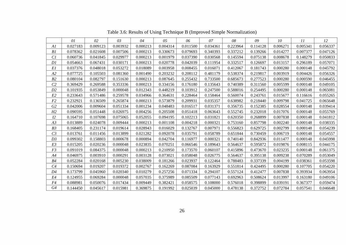
Table 3.6: Results of Using Technique B (Improved Simple Normalization) 01 02 03 04 05 06 07 08 09 10 11 12


26

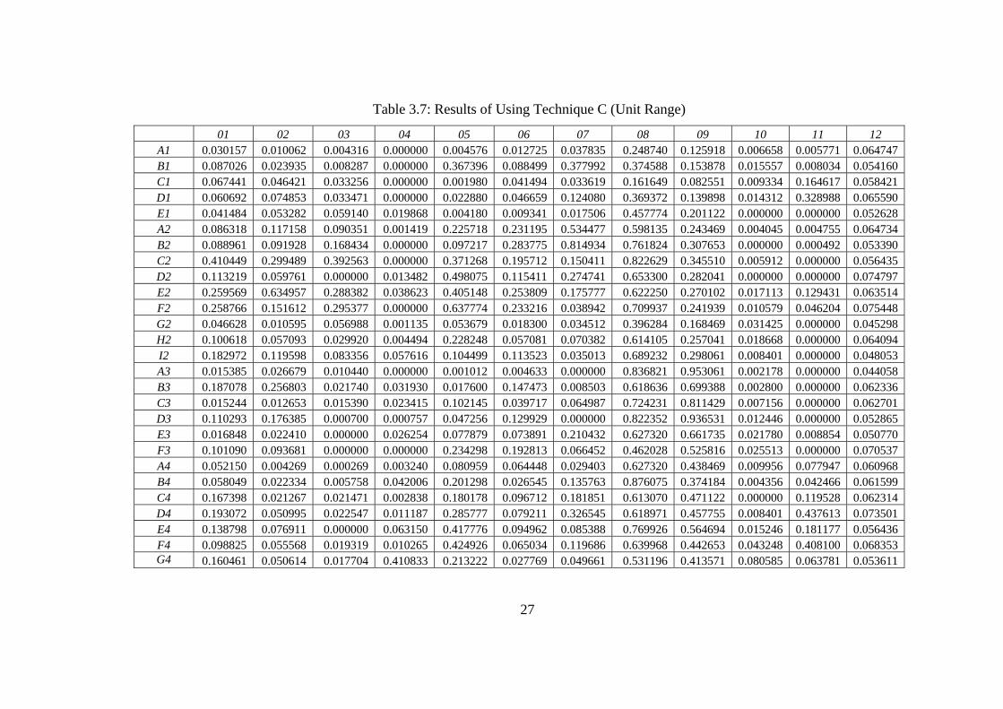
Table 3.7: Results of Using Technique C (Unit Range)

01 02 03 04 05 06 07 08 09 10 11 12 A1 0.030157 0.010062 0.004316 0.000000 0.004576 0.012725 0.037835 0.248740 0.125918 0.006658 0.005771 0.064747 B1 0.087026 0.023935 0.008287 0.000000 0.367396 0.088499 0.377992 0.374588 0.153878 0.015557 0.008034 0.054160 C1 0.067441 0.046421 0.033256 0.000000 0.001980 0.041494 0.033619 0.161649 0.082551 0.009334 0.164617 0.058421 D1 0.060692 0.074853 0.033471 0.000000 0.022880 0.046659 0.124080 0.369372 0.139898 0.014312 0.328988 0.065590 E1 0.041484 0.053282 0.059140 0.019868 0.004180 0.009341 0.017506 0.457774 0.201122 0.000000 0.000000 0.052628 A2 0.086318 0.117158 0.090351 0.001419 0.225718 0.231195 0.534477 0.598135 0.243469 0.004045 0.004755 0.064734 B2 0.088961 0.091928 0.168434 0.000000 0.097217 0.283775 0.814934 0.761824 0.307653 0.000000 0.000492 0.053390 C2 0.410449 0.299489 0.392563 0.000000 0.371268 0.195712 0.150411 0.822629 0.345510 0.005912 0.000000 0.056435 D2 0.113219 0.059761 0.000000 0.013482 0.498075 0.115411 0.274741 0.653300 0.282041 0.000000 0.000000 0.074797 E2 0.259569 0.634957 0.288382 0.038623 0.405148 0.253809 0.175777 0.622250 0.270102 0.017113 0.129431 0.063514 F2 0.258766 0.151612 0.295377 0.000000 0.637774 0.233216 0.038942 0.709937 0.241939 0.010579 0.046204 0.075448 G2 0.046628 0.010595 0.056988 0.001135 0.053679 0.018300 0.034512 0.396284 0.168469 0.031425 0.000000 0.045298 H2 0.100618 0.057093 0.029920 0.004494 0.228248 0.057081 0.070382 0.614105 0.257041 0.018668 0.000000 0.064094 I2 0.182972 0.119598 0.083356 0.057616 0.104499 0.113523 0.035013 0.689232 0.298061 0.008401 0.000000 0.048053 A3 0.015385 0.026679 0.010440 0.000000 0.001012 0.004633 0.000000 0.836821 0.953061 0.002178 0.000000 0.044058 B3 0.187078 0.256803 0.021740 0.031930 0.017600 0.147473 0.008503 0.618636 0.699388 0.002800 0.000000 0.062336 C3 0.015244 0.012653 0.015390 0.023415 0.102145 0.039717 0.064987 0.724231 0.811429 0.007156 0.000000 0.062701 D3 0.110293 0.176385 0.000700 0.000757 0.047256 0.129929 0.000000 0.822352 0.936531 0.012446 0.000000 0.052865 E3 0.016848 0.022410 0.000000 0.026254 0.077879 0.073891 0.210432 0.627320 0.661735 0.021780 0.008854 0.050770 F3 0.101090 0.093681 0.000000 0.000000 0.234298 0.192813 0.066452 0.462028 0.525816 0.025513 0.000000 0.070537 A4 0.052150 0.004269 0.000269 0.003240 0.080959 0.064448 0.029403 0.627320 0.438469 0.009956 0.077947 0.060968 B4 0.058049 0.022334 0.005758 0.042006 0.201298 0.026545 0.135763 0.876075 0.374184 0.004356 0.042466 0.061599 C4 0.167398 0.021267 0.021471 0.002838 0.180178 0.096712 0.181851 0.613070 0.471122 0.000000 0.119528 0.062314 D4 0.193072 0.050995 0.022547 0.011187 0.285777 0.079211 0.326545 0.618971 0.457755 0.008401 0.437613 0.073501 E4 0.138798 0.076911 0.000000 0.063150 0.417776 0.094962 0.085388 0.769926 0.564694 0.015246 0.181177 0.056436 F4 0.098825 0.055568 0.019319 0.010265 0.424926 0.065034 0.119686 0.639968 0.442653 0.043248 0.408100 0.068353 G4 0.160461 0.050614 0.017704 0.410833 0.213222 0.027769 0.049661 0.531196 0.413571 0.080585 0.063781 0.053611

27

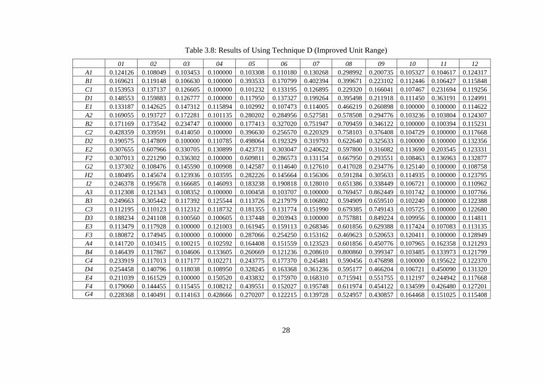
Table 3.8: Results of Using Technique D (Improved Unit Range) 01 02 03 04 05 06 07 08 09 10 11 12


28

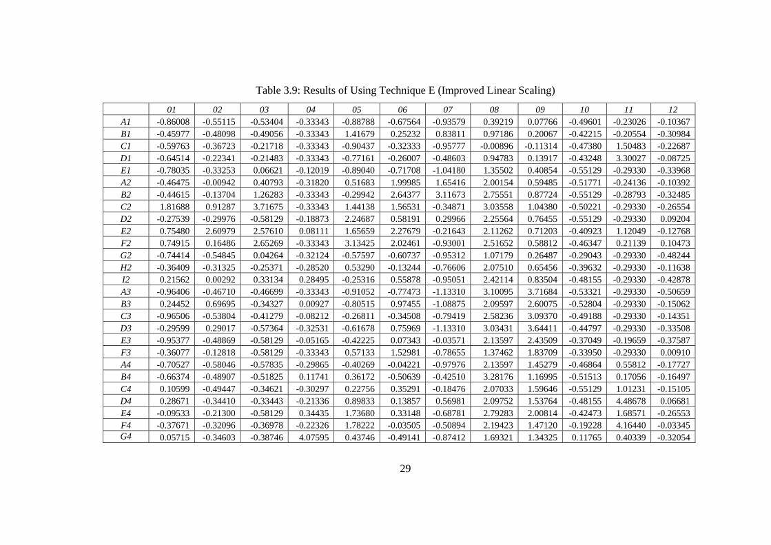
Table 3.9: Results of Using Technique E (Improved Linear Scaling) 01 02 03 04 05 06 07 08 09 10 11 12

A1 -0.86008 -0.55115 -0.53404 -0.33343 -0.88788 -0.67564 -0.93579 0.39219 0.07766 -0.49601 -0.23026 -0.10367 B1 -0.45977 -0.48098 -0.49056 -0.33343 1.41679 0.25232 0.83811 0.97186 0.20067 -0.42215 -0.20554 -0.30984 C1 -0.59763 -0.36723 -0.21718 -0.33343 -0.90437 -0.32333 -0.95777 -0.00896 -0.11314 -0.47380 1.50483 -0.22687 D1 -0.64514 -0.22341 -0.21483 -0.33343 -0.77161 -0.26007 -0.48603 0.94783 0.13917 -0.43248 3.30027 -0.08725 E1 -0.78035 -0.33253 0.06621 -0.12019 -0.89040 -0.71708 -1.04180 1.35502 0.40854 -0.55129 -0.29330 -0.33968 A2 -0.46475 -0.00942 0.40793 -0.31820 0.51683 1.99985 1.65416 2.00154 0.59485 -0.51771 -0.24136 -0.10392 B2 -0.44615 -0.13704 1.26283 -0.33343 -0.29942 2.64377 3.11673 2.75551 0.87724 -0.55129 -0.28793 -0.32485 C2 1.81688 0.91287 3.71675 -0.33343 1.44138 1.56531 -0.34871 3.03558 1.04380 -0.50221 -0.29330 -0.26554 D2 -0.27539 -0.29976 -0.58129 -0.18873 2.24687 0.58191 0.29966 2.25564 0.76455 -0.55129 -0.29330 0.09204 E2 0.75480 2.60979 2.57610 0.08111 1.65659 2.27679 -0.21643 2.11262 0.71203 -0.40923 1.12049 -0.12768 F2 0.74915 0.16486 2.65269 -0.33343 3.13425 2.02461 -0.93001 2.51652 0.58812 -0.46347 0.21139 0.10473 G2 -0.74414 -0.54845 0.04264 -0.32124 -0.57597 -0.60737 -0.95312 1.07179 0.26487 -0.29043 -0.29330 -0.48244 H2 -0.36409 -0.31325 -0.25371 -0.28520 0.53290 -0.13244 -0.76606 2.07510 0.65456 -0.39632 -0.29330 -0.11638 I2 0.21562 0.00292 0.33134 0.28495 -0.25316 0.55878 -0.95051 2.42114 0.83504 -0.48155 -0.29330 -0.42878 A3 -0.96406 -0.46710 -0.46699 -0.33343 -0.91052 -0.77473 -1.13310 3.10095 3.71684 -0.53321 -0.29330 -0.50659 B3 0.24452 0.69695 -0.34327 0.00927 -0.80515 0.97455 -1.08875 2.09597 2.60075 -0.52804 -0.29330 -0.15062 C3 -0.96506 -0.53804 -0.41279 -0.08212 -0.26811 -0.34508 -0.79419 2.58236 3.09370 -0.49188 -0.29330 -0.14351 D3 -0.29599 0.29017 -0.57364 -0.32531 -0.61678 0.75969 -1.13310 3.03431 3.64411 -0.44797 -0.29330 -0.33508 E3 -0.95377 -0.48869 -0.58129 -0.05165 -0.42225 0.07343 -0.03571 2.13597 2.43509 -0.37049 -0.19659 -0.37587 F3 -0.36077 -0.12818 -0.58129 -0.33343 0.57133 1.52981 -0.78655 1.37462 1.83709 -0.33950 -0.29330 0.00910 A4 -0.70527 -0.58046 -0.57835 -0.29865 -0.40269 -0.04221 -0.97976 2.13597 1.45279 -0.46864 0.55812 -0.17727 B4 -0.66374 -0.48907 -0.51825 0.11741 0.36172 -0.50639 -0.42510 3.28176 1.16995 -0.51513 0.17056 -0.16497 C4 0.10599 -0.49447 -0.34621 -0.30297 0.22756 0.35291 -0.18476 2.07033 1.59646 -0.55129 1.01231 -0.15105 D4 0.28671 -0.34410 -0.33443 -0.21336 0.89833 0.13857 0.56981 2.09752 1.53764 -0.48155 4.48678 0.06681 E4 -0.09533 -0.21300 -0.58129 0.34435 1.73680 0.33148 -0.68781 2.79283 2.00814 -0.42473 1.68571 -0.26553 F4 -0.37671 -0.32096 -0.36978 -0.22326 1.78222 -0.03505 -0.50894 2.19423 1.47120 -0.19228 4.16440 -0.03345 G4 0.05715 -0.34603 -0.38746 4.07595 0.43746 -0.49141 -0.87412 1.69321 1.34325 0.11765 0.40339 -0.32054

29

In order to evaluate which is the best data conversion techniques, the results/output

obtained are used as input to the ANN model for prediction purposes, described in

the following chapter.

3.4 Summary

This chapter describes the first and second objectives of this project; that is to

identify the format and values for input parameters affecting the rice yield and

to investigate, design and develop data conversion and reduction algorithm for

input parameters affecting rice yield. As for the input parameters, there

altogether thirty-five (35) parameters, however the most significant ones are

only eleven (11) parameters. The values are all numeric.

Data conversion is necessary to prepare the input data so that it is suitable to be

accepted by the ANN Model. Two (2) approaches are evaluated. The first

approach consists of three (3) methods namely; maximum and minimum

values, mean and standard deviation and pricipal component analysis

technique. The second approach consists of six (6) techniques namely; simple

normalization, improved simple normalization, unit range technique, improved

unit range and improved linear scaling. Evaluation of these techniques are

performed in the next chapter using ANN model to perform the rice yield

prediction.

30

46

CHAPTER 5

IDSS ARCHITECTURE AND PROTOTYPE 5.1 Introduction

This chapter will finally describe the architecture and the prototype of the IDSS. The

IDSS architecture comprises of the previous modules explained before. The IDSS

prototype is the final output desired in this research project. The prototype consists of 3

main modules/sub-system namely; IndiCA1, IndiCA2 and Pest Management. IndiCA1

helps farmers to plan paddy planting activities. IndiCA2 help farmers to predict rice

yield by entering values of the relevant parameters. Pest Management sub-system helps

farmers to control pests in their paddy fields.

This chapter starts with Section 5.2 on IDSS Architecture, followed by Section 5.3 on

IDSS Prototype and the chapter ends with a summary in Section 5.4.

5.2 IDSS Architecture

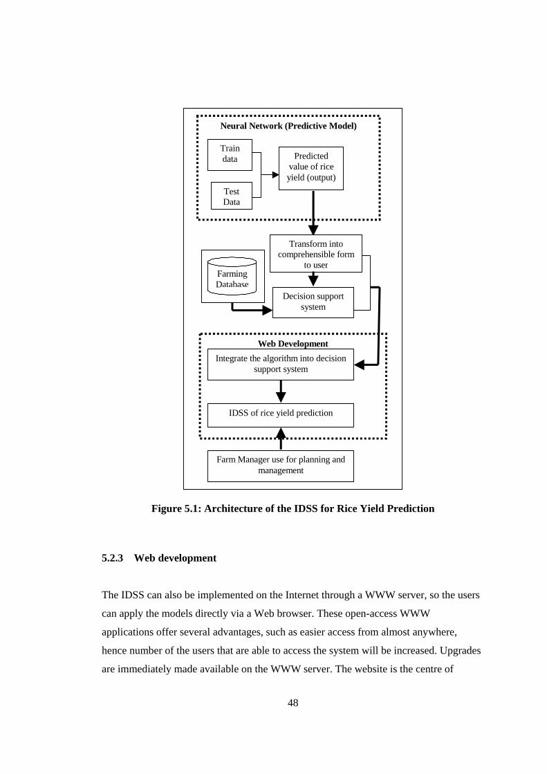
The architecture of the IDSS for rice yield prediction is shown in Figure 5.1. Five (5)

major components are integrated to form the architecture: The components are;(1) the

predictive model (2) the decision support system (3) the web development (4) the

47

farming database to store rice parameters and (5) the user. Each of the components is

described below.

5.2.1 Predictive model

This is the model that was used to perform the rice yield prediction task. The factors that

affect rice yield act as the model input. The model was described in detail in Chapter 4.

The output was presented to the user after going through the user application

component.

5.2.2 Decision support system This component is used to control the management of decision-making information.

Information about paddy, crop characteristics, and affected factors of rice yield is

managed by this sub-system. The sub-system also contain the interfaces that helps

farmers or farm managers to input data, view the output that is generated by the

intelligent component and to perform what if analysis. Hence the user can culminate

decisions to maximize rice production.

48

Figure 5.1: Architecture of the IDSS for Rice Yield Prediction

5.2.3 Web development The IDSS can also be implemented on the Internet through a WWW server, so the users

can apply the models directly via a Web browser. These open-access WWW

applications offer several advantages, such as easier access from almost anywhere,

hence number of the users that are able to access the system will be increased. Upgrades

are immediately made available on the WWW server. The website is the centre of

Neural Network (Predictive Model)

Web Development

Farm Manager use for planning and management

Train data

Test Data

Predicted value of rice yield (output)

Transform into comprehensible form

to user

Decision support system

Integrate the algorithm into decision support system

IDSS of rice yield prediction

Farming Database

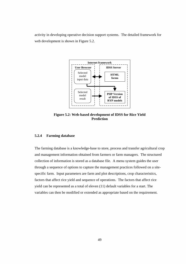
49

activity in developing operative decision support systems. The detailed framework for

web development is shown in Figure 5.2.

Internet framework

User Browser IDSS Server

Selected model

input data

Selected model result

HTML forms

PHP Version of IDSS of

RYP models

Figure 5.2: Web-based development of IDSS for Rice Yield Prediction

5.2.4 Farming database The farming database is a knowledge-base to store, process and transfer agricultural crop

and management information obtained from farmers or farm managers. The structured

collection of information is stored as a database file. A menu system guides the user

through a sequence of options to capture the management practices followed on a site-

specific farm. Input parameters are farm and plot descriptions, crop characteristics,

factors that affect rice yield and sequence of operations. The factors that affect rice

yield can be represented as a total of eleven (11) default variables for a start. The

variables can then be modified or extended as appropriate based on the requirement.

50

5.2.5 User The user communicates with and commands the IDSS through this component. The

user is considered as a component of the system. Researchers claim that some of the

unique contributions of IDSS originates from the rigorous interaction between the

computer and the decision maker [14]. Through this component the user can control the

management of their farm and also obtain information on the predicted yield of their

farm.

5.3 IndiCA – the IDSS Prototype The IDSS Prototype-IndiCA consists of the following subsystems; IndiCA1, IndiCA2

and Pest Management as depicted in Figure 5.3.

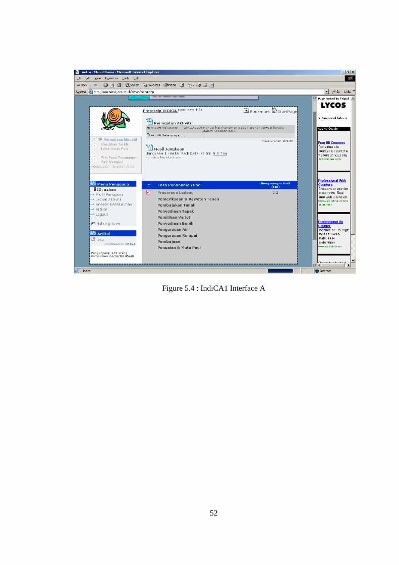
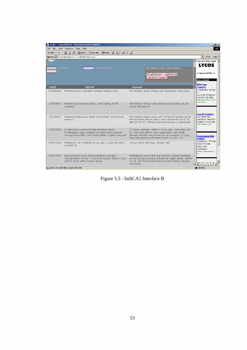
IndiCA1 help farmers to plan paddy planting activities. Here user/farmers only need to

enter the seedling planting date. The system will then create a complete task schedule.

For instance, what is the suitable date to drain out water from the paddy fields.

Examples of associated interfaces regarding IndiCA1 are depicted in Figure 5.4 and

Figure 5.5.

IndiCA2 help farmers to predict rice yield by entering values for the following

parameters such as weed (rumpai, rusiga, daun lebar), pest (rats, worms, bena perang),

diseases (bacteria, jalur daun merah, hawar seludang), wind paddy and lodging

(kerebahan). Based on the values entered, IndiCA2 able to predict the rice yield to be

obtained.

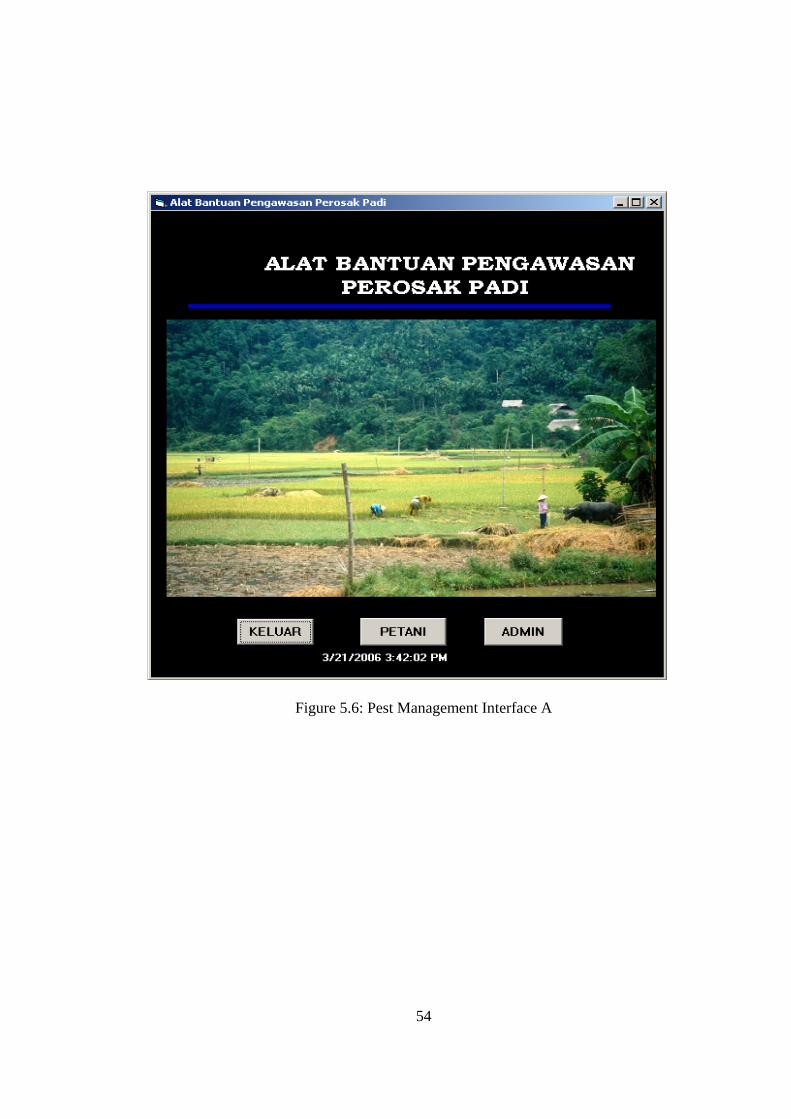
Pest Management sub-system helps farmers to control pests in their paddy fields. The

interfaces for this sub-system are shown in Figure 5.6 and Figure 5.7

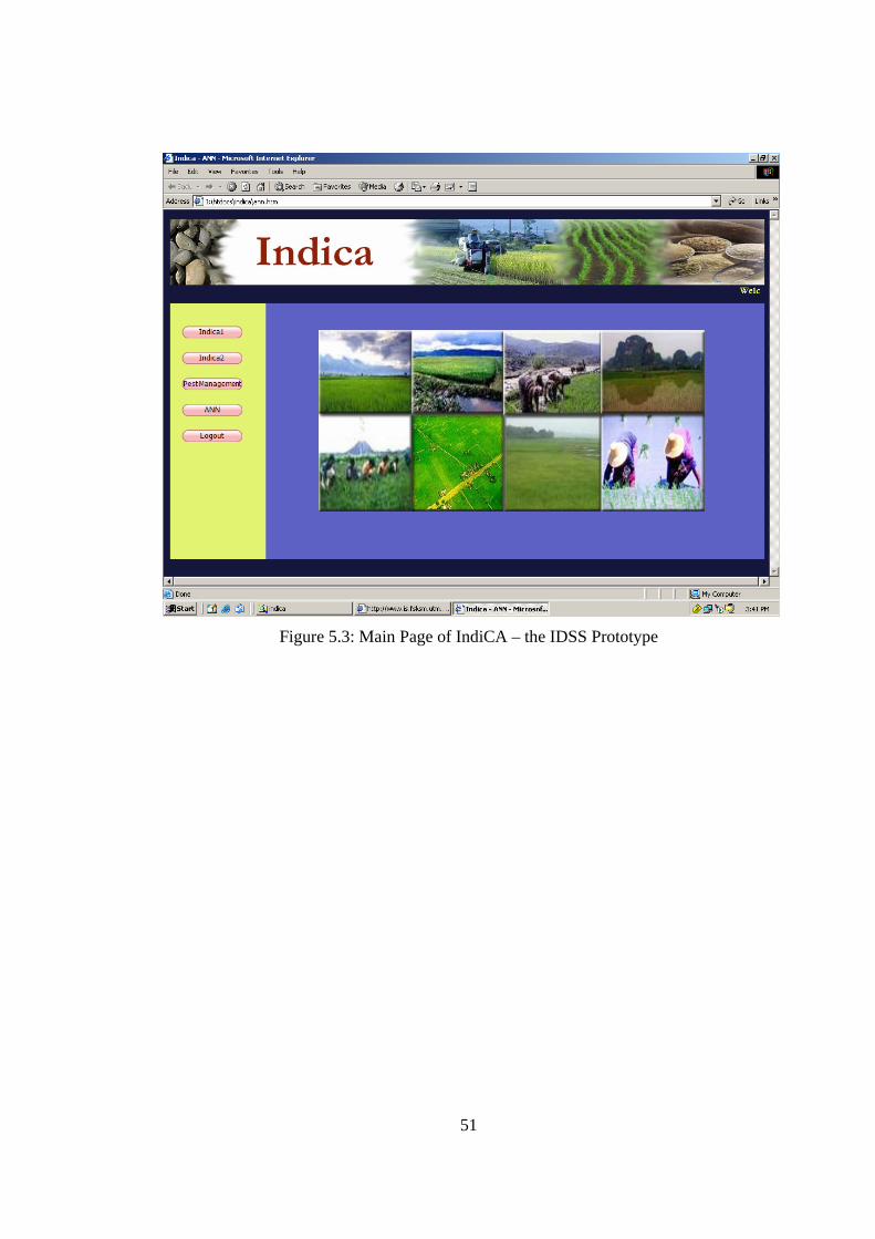
51

Figure 5.3: Main Page of IndiCA – the IDSS Prototype

52

Figure 5.4 : IndiCA1 Interface A

53

Figure 5.5 : IndiCA1 Interface B

54

Figure 5.6: Pest Management Interface A

55

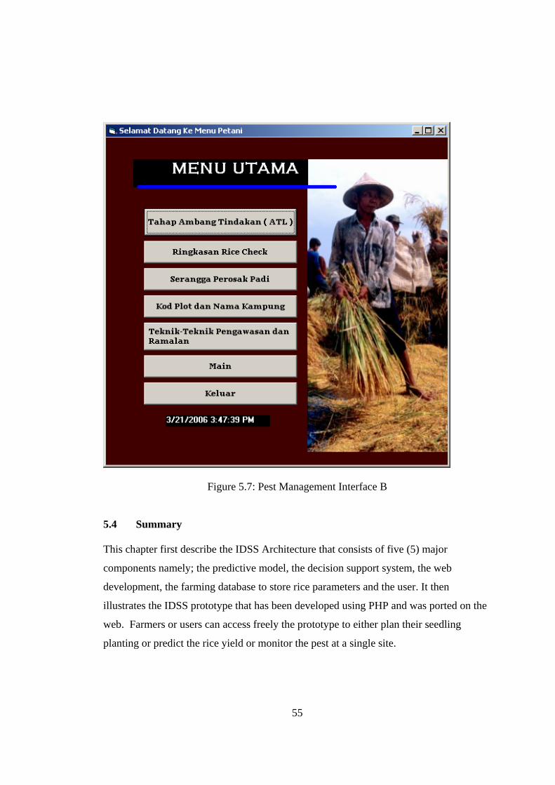
Figure 5.7: Pest Management Interface B 5.4 Summary This chapter first describe the IDSS Architecture that consists of five (5) major

components namely; the predictive model, the decision support system, the web

development, the farming database to store rice parameters and the user. It then

illustrates the IDSS prototype that has been developed using PHP and was ported on the

web. Farmers or users can access freely the prototype to either plan their seedling

planting or predict the rice yield or monitor the pest at a single site.

31

CHAPTER 4

ARTIFICIAL NEURAL NETWORK MODEL

4.1 Introduction

The artificial neural network (ANN) is chosen as the intelligent component in the IDSS.

Hence this chapter describes the processes involved in using the ANN for the purposes

of prediction. There are a variety of ANN models available, however two (2) types are

found to be suitable for prediction purposes that is Back-propagation (BP) and Radial

Basis Function (RBF) ANN models.

This chapter starts with Section 4.2 on Modeling the Rice Yield Data, Section 4.3 is on

ANN parameters and Architecture. Section 4.4 discusses Performance of Conversion

Algorithms using BP ANN Model, Section 4.5 is on Performance of Enhanced BP ANN

Model. Section 4.6 discusses the Performance of RBF ANN. Section 4.7 iterate

Gradient Descent with Momentum and Adaptive Learning Backpropagation and this

chapter ended with a summary in Section 4.8.

32

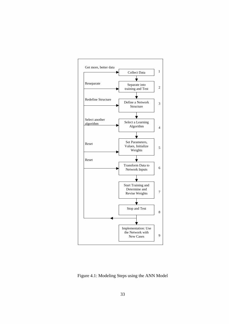
4.2 Modeling the Rice Yield Data The development of ANN model consists of 6 steps as referred in [12] depicted in

Figure 1. In Step 1 the data to be used for training are collected from Muda Agricultural

Development Authority (MADA) as described in Chapter 3.

In Step 2 the training data need to be identified, and plan must be made for testing the

performance of the network. The collected data are separated into training and test sets.

80% of the data are utilized for training the ANN Model and 20% of the data are

reserved for testing. Out of 378 total set data, 302 sets are chosen for training and 76 set

are used for prediction.

In Step 3 and 4 a network architecture and a learning method are selected.

Step 5 is the initialization of the network weights and parameters, followed by

modification of the parameters such as momentum, learning rate and number of neuron

in the hidden layer as performance feedback is received. Since these are 11 factors that

affect yield, hence the number of node in the input layer is 11. The number of node in

the output layer is 1 represent the rice yield. Several training is done to obtain the

suitable number of nodes in the hidden layer,momentum values and learning rate.

The activities in Step 6, is to convert/transform the input data into the type and format

required by the ANN Model. Several conversion algorithms are explored as explained in

the previous chapter, Chapter 3.

In Step 7 and Step 8, training and prediction are done. Two artificial neural network

models are utilized namely; Back Propagation Neural Network Model and its

enhancement and Radial Basis Function Neural Network Model (RBF).

33

Get more, better data 1 1 Reseparate

2 Redefine Structure

3 Select another algorithm

4

Reset 5

Reset

6

7

8

9

Collect Data

Separate into training and Test

Define a Network Structure

Select a Learning Algorithm

Set Parameters, Values, Initialize

Weights

Implementation: Use the Network with

New Cases

Transform Data to Network Inputs

Start Training and Determine and Revise Weights

Stop and Test

Figure 4.1: Modeling Steps using the ANN Model

34

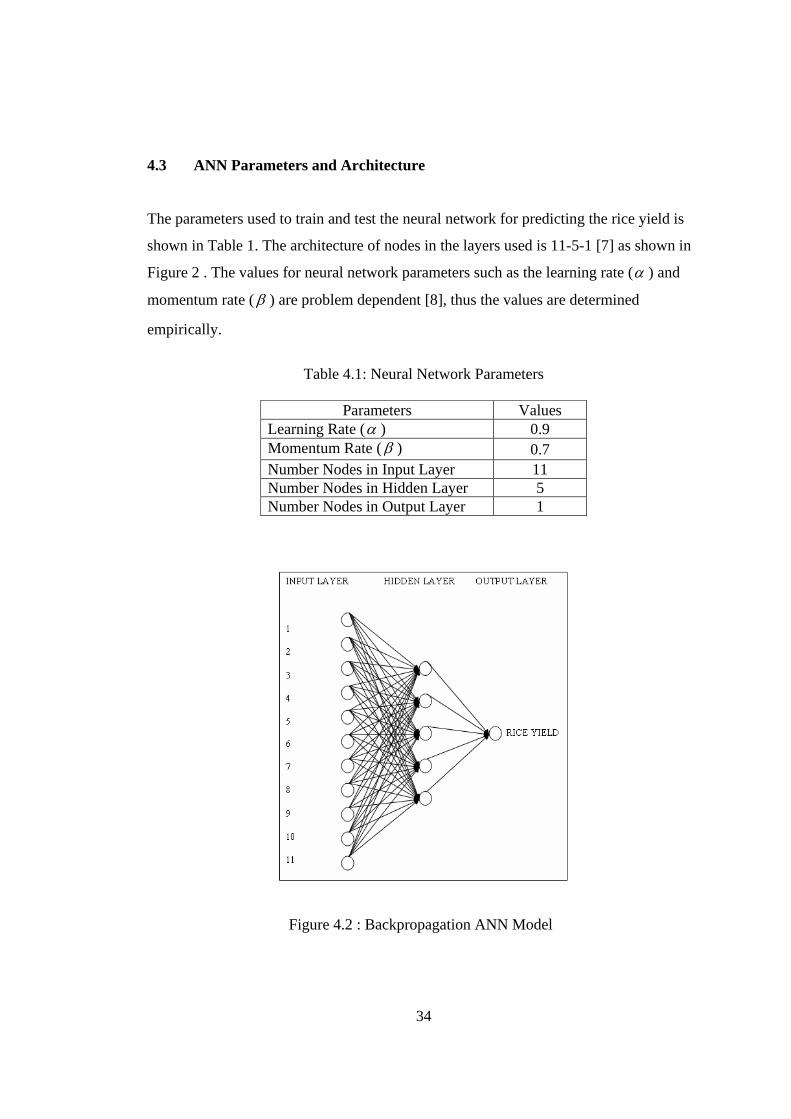
4.3 ANN Parameters and Architecture The parameters used to train and test the neural network for predicting the rice yield is

shown in Table 1. The architecture of nodes in the layers used is 11-5-1 [7] as shown in

Figure 2 . The values for neural network parameters such as the learning rate (α ) and

momentum rate ( β ) are problem dependent [8], thus the values are determined

empirically.

Table 4.1: Neural Network Parameters

Parameters Values

Learning Rate (α ) 0.9 Momentum Rate (β ) 0.7 Number Nodes in Input Layer 11 Number Nodes in Hidden Layer 5 Number Nodes in Output Layer 1

Figure 4.2 : Backpropagation ANN Model

35

4.4 Performance of Conversion Algorithms using BP ANN Model The results obtained after the data convertion process is implemented on the input data

as shown in Figure 3.5 to Figure 3.9 in Chapter 3 is feed into the BP ANN model for

both training and testing. Outputs from the training process will be used to identify the

deviation between network outputs and actual outputs for each technique using the

following equations.

Deviation = dataofno

outoutdataofno

itn

__

__

1∑=

− , outn > outt (1)

Deviation = dataofno

outoutdataofno

int

__

__

1∑=

− , outt > outn (2)

where,

outn - the network output outt - the target output

In order to obtain the mean deviation for each technique, all the deviations computed

using equation (1) and equation (2) between every network outputs and actual outputs

are summed up and divided by the total number of the data.

Mean Deviation = taNumberofDa

utActualOutpputNetworkOut∑ − )( (3)

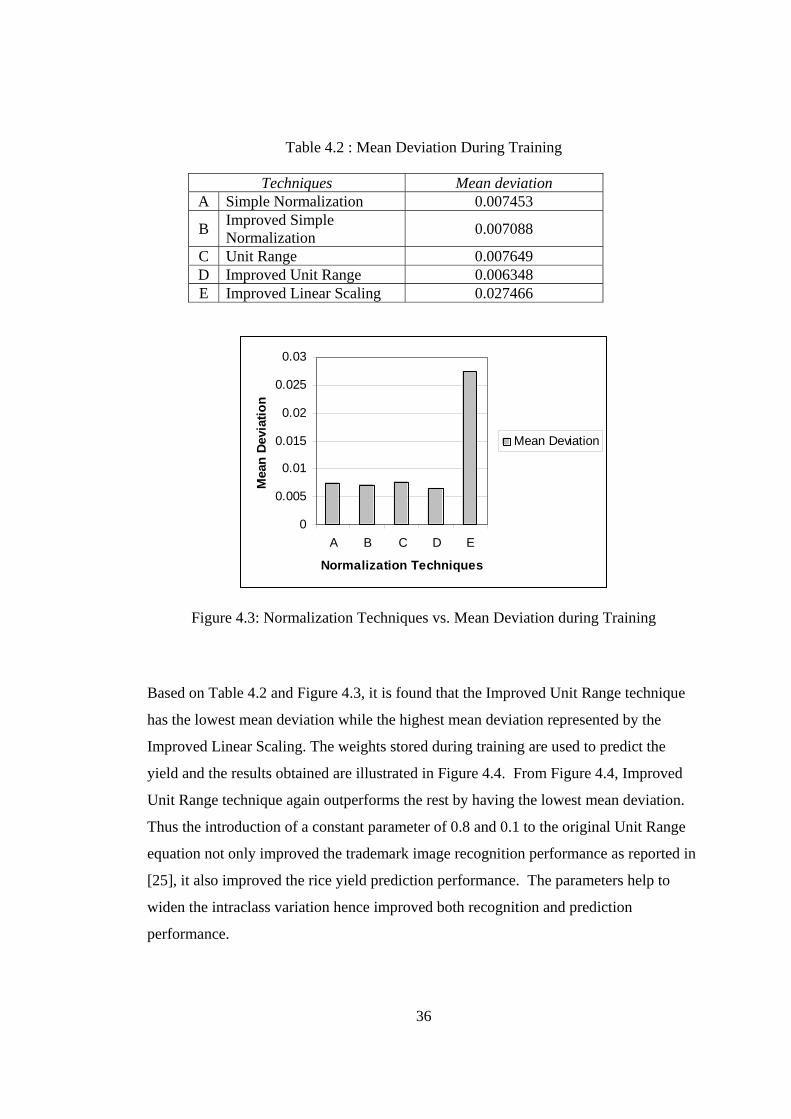
Table 4.2 shows the mean deviation obtained when the algorithm has converged during

training session. Graphs of normalization techniques are plotted against mean deviation

as depicted in Figure 4.3.

36

Table 4.2 : Mean Deviation During Training

0

0.005

0.01

0.015

0.02

0.025

0.03

A B C D E

Normalization Techniques

Mea

n De

viat

ion

Mean Deviation

Figure 4.3: Normalization Techniques vs. Mean Deviation during Training

Based on Table 4.2 and Figure 4.3, it is found that the Improved Unit Range technique

has the lowest mean deviation while the highest mean deviation represented by the

Improved Linear Scaling. The weights stored during training are used to predict the

yield and the results obtained are illustrated in Figure 4.4. From Figure 4.4, Improved

Unit Range technique again outperforms the rest by having the lowest mean deviation.

Thus the introduction of a constant parameter of 0.8 and 0.1 to the original Unit Range

equation not only improved the trademark image recognition performance as reported in

[25], it also improved the rice yield prediction performance. The parameters help to

widen the intraclass variation hence improved both recognition and prediction

performance.

Techniques Mean deviation A Simple Normalization 0.007453

B Improved Simple Normalization 0.007088

C Unit Range 0.007649 D Improved Unit Range 0.006348 E Improved Linear Scaling 0.027466

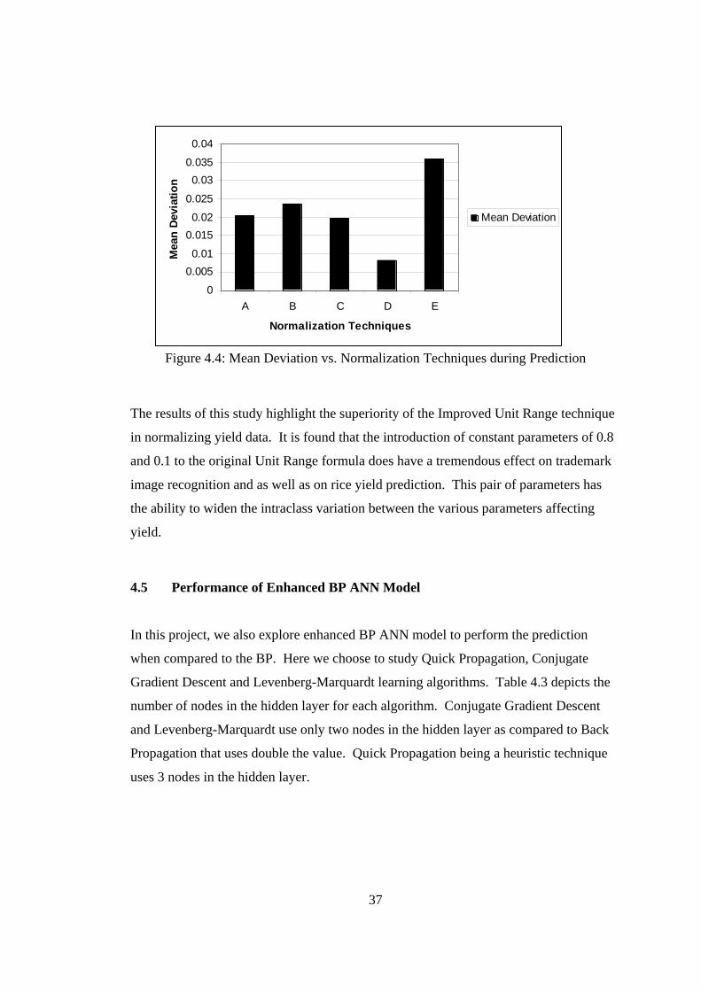
37

0

0.0050.01

0.0150.02

0.025

0.030.035

0.04

A B C D E

Normalization Techniques

Mea

n De

viat

ion

Mean Deviation

Figure 4.4: Mean Deviation vs. Normalization Techniques during Prediction

The results of this study highlight the superiority of the Improved Unit Range technique

in normalizing yield data. It is found that the introduction of constant parameters of 0.8

and 0.1 to the original Unit Range formula does have a tremendous effect on trademark

image recognition and as well as on rice yield prediction. This pair of parameters has

the ability to widen the intraclass variation between the various parameters affecting

yield.

4.5 Performance of Enhanced BP ANN Model In this project, we also explore enhanced BP ANN model to perform the prediction

when compared to the BP. Here we choose to study Quick Propagation, Conjugate

Gradient Descent and Levenberg-Marquardt learning algorithms. Table 4.3 depicts the

number of nodes in the hidden layer for each algorithm. Conjugate Gradient Descent

and Levenberg-Marquardt use only two nodes in the hidden layer as compared to Back

Propagation that uses double the value. Quick Propagation being a heuristic technique

uses 3 nodes in the hidden layer.

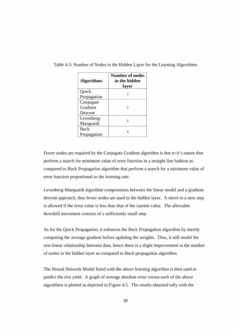
38

Table 4.3: Number of Nodes in the Hidden Layer for the Learning Algorithms

Algorithms Number of nodes

in the hidden layer

Quick Propagation

3

Conjugate Gradient Descent

2

Levenberg- Marquardt

2

Back Propagation

4

Fewer nodes are required by the Conjugate Gradient algorithm is due to it’s nature that

perform a search for minimum value of error function in a straight line fashion as

compared to Back Propagation algorithm that perform a search for a minimum value of

error function proportional to the learning rate.

Levenberg-Marquardt algorithm compromises between the linear model and a gradient-

descent approach, thus fewer nodes are used in the hidden layer. A move to a next step

is allowed if the error value is less than that of the current value. The allowable

downhill movement consists of a sufficiently small step.

As for the Quick Propagation, it enhances the Back Propagation algorithm by merely

computing the average gradient before updating the weights. Thus, it still model the

non-linear relationship between data, hence there is a slight improvement in the number

of nodes in the hidden layer as compared to Back-propagation algorithm.

The Neural Network Model fitted with the above learning algorithm is then used to

predict the rice yield. A graph of average absolute error versus each of the above

algorithms is plotted as depicted in Figure 4.5. The results obtained tally with the

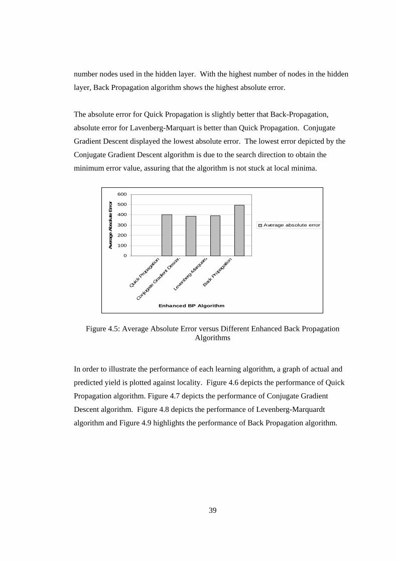
39

number nodes used in the hidden layer. With the highest number of nodes in the hidden

layer, Back Propagation algorithm shows the highest absolute error.

The absolute error for Quick Propagation is slightly better that Back-Propagation,

absolute error for Lavenberg-Marquart is better than Quick Propagation. Conjugate

Gradient Descent displayed the lowest absolute error. The lowest error depicted by the

Conjugate Gradient Descent algorithm is due to the search direction to obtain the

minimum error value, assuring that the algorithm is not stuck at local minima.

0

100

200

300

400

500

600

Quick P

ropa

gatio

n

Conju

gate

Gradie

nt D

esce

n

Leve

nberg-Marqu

ardt

Back

Propa

gatio

n

Enhanced BP Algorithm

Ave

rage

Abs

olut

e Err

or

Average absolute error

Figure 4.5: Average Absolute Error versus Different Enhanced Back Propagation Algorithms

In order to illustrate the performance of each learning algorithm, a graph of actual and

predicted yield is plotted against locality. Figure 4.6 depicts the performance of Quick

Propagation algorithm. Figure 4.7 depicts the performance of Conjugate Gradient

Descent algorithm. Figure 4.8 depicts the performance of Levenberg-Marquardt

algorithm and Figure 4.9 highlights the performance of Back Propagation algorithm.

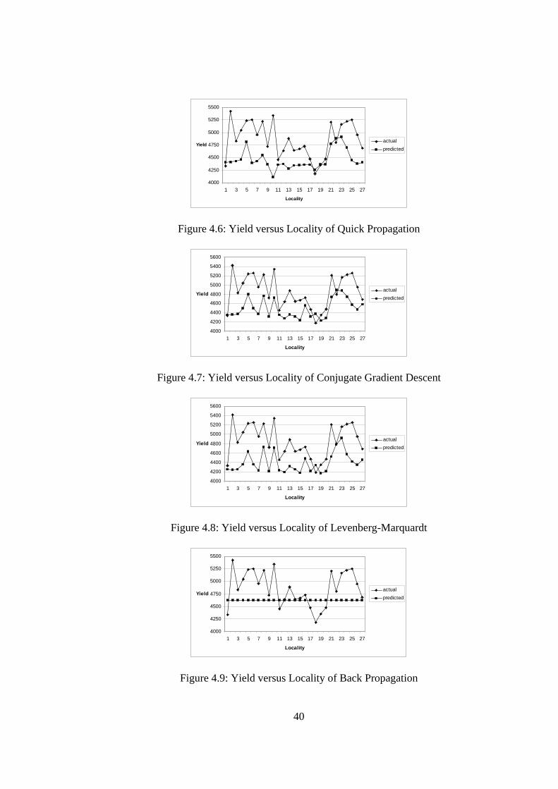
40

4000

4250

4500

4750

5000

5250

5500

1 3 5 7 9 11 13 15 17 19 21 23 25 27

Locality

Yieldactualpredicted

Figure 4.6: Yield versus Locality of Quick Propagation

4000

4200

4400

4600

4800

5000

5200

5400

5600

1 3 5 7 9 11 13 15 17 19 21 23 25 27

Locality


Figure 4.7: Yield versus Locality of Conjugate Gradient Descent

4000

4200

4400

4600

4800

5000

5200

5400

5600

1 3 5 7 9 11 13 15 17 19 21 23 25 27

Locality


Figure 4.8: Yield versus Locality of Levenberg-Marquardt

4000

4250

4500

4750

5000

5250

5500

1 3 5 7 9 11 13 15 17 19 21 23 25 27

Locality


Figure 4.9: Yield versus Locality of Back Propagation

41

Based on Figure 4.6 to Figure 4.9, Conjugate Gradient Descent algorithm portrays the

best performance as compared to the other. The next to it is Lavenberg-Marquart and

then Quick Propagation. Back Propagation algorithm failed to produce the desired

output due the major problem of being stuck at local minima. The outstanding

performance of the Conjugate Gradient Descent algorithm is due to the strategy that

successive weight correction steps are orthogonal to the gradient. Thus attributing it to

exhibit a quadratic convergence property that avoid the local minima phenomena.

Lavenberg-Marquart is another alternative to choose in training the Neural Network for

rice yield prediction. Its superiority as compared to Back Propagation algorithm is that

the training is based on second-order derivative approach that avoid local minima

problem and exhibit a faster convergence. However Lavenberg-Marquart algorithm has

a major drawback that it requires the storage of some matrices that can be quite large for

this kind of problems. Thus, when comparison is performed between Lavenberg-

Marquart and Conjugate Gradient Descent, Conjugate Gradient Descent wins.

4.6 Gradient Descent with Momentum and Adaptive Learning

Backpropagation

Another test run with the same data, using gradient descent and the result of the training

process is shown in Figure 4.11. From the results acquired, it can be seen that the

training process on the network using backpropagation technique failed to reach 0.001

targets after 5000 epochs.

Mean square errors represent network’s performance of the MLP network and have

been set to 0.001. The smaller mean square error generate, the better network will

produce. As shown in Table 4.5, after 5000 iterations, mean square error just reaches

0.041227.

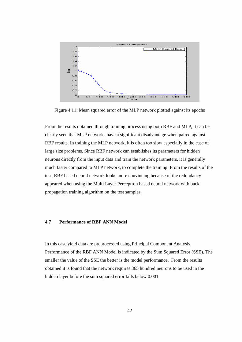
42

Figure 4.11: Mean squared error of the MLP network plotted against its epochs From the results obtained through training process using both RBF and MLP, it can be

clearly seen that MLP networks have a significant disadvantage when paired against

RBF results. In training the MLP network, it is often too slow especially in the case of

large size problems. Since RBF network can establishes its parameters for hidden

neurons directly from the input data and train the network parameters, it is generally

much faster compared to MLP network, to complete the training. From the results of the

test, RBF based neural network looks more convincing because of the redundancy

appeared when using the Multi Layer Perceptron based neural network with back

propagation training algorithm on the test samples.

4.7 Performance of RBF ANN Model In this case yield data are preprocessed using Principal Component Analysis.

Performance of the RBF ANN Model is indicated by the Sum Squared Error (SSE). The

smaller the value of the SSE the better is the model performance. From the results

obtained it is found that the network requires 365 hundred neurons to be used in the

hidden layer before the sum squared error falls below 0.001

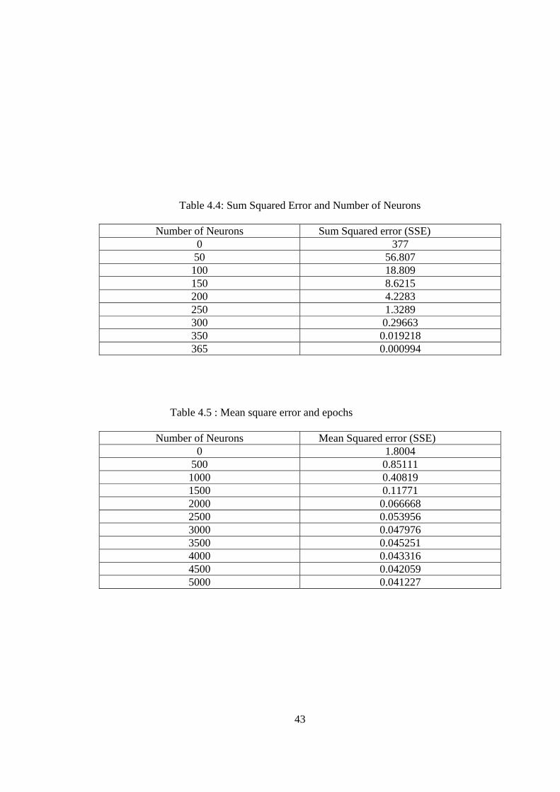
43

Table 4.4: Sum Squared Error and Number of Neurons

Number of Neurons Sum Squared error (SSE) 0 377

50 56.807 100 18.809 150 8.6215 200 4.2283 250 1.3289 300 0.29663 350 0.019218 365 0.000994

Table 4.5 : Mean square error and epochs

Number of Neurons Mean Squared error (SSE) 0 1.8004

500 0.85111 1000 0.40819 1500 0.11771 2000 0.066668 2500 0.053956 3000 0.047976 3500 0.045251 4000 0.043316 4500 0.042059 5000 0.041227

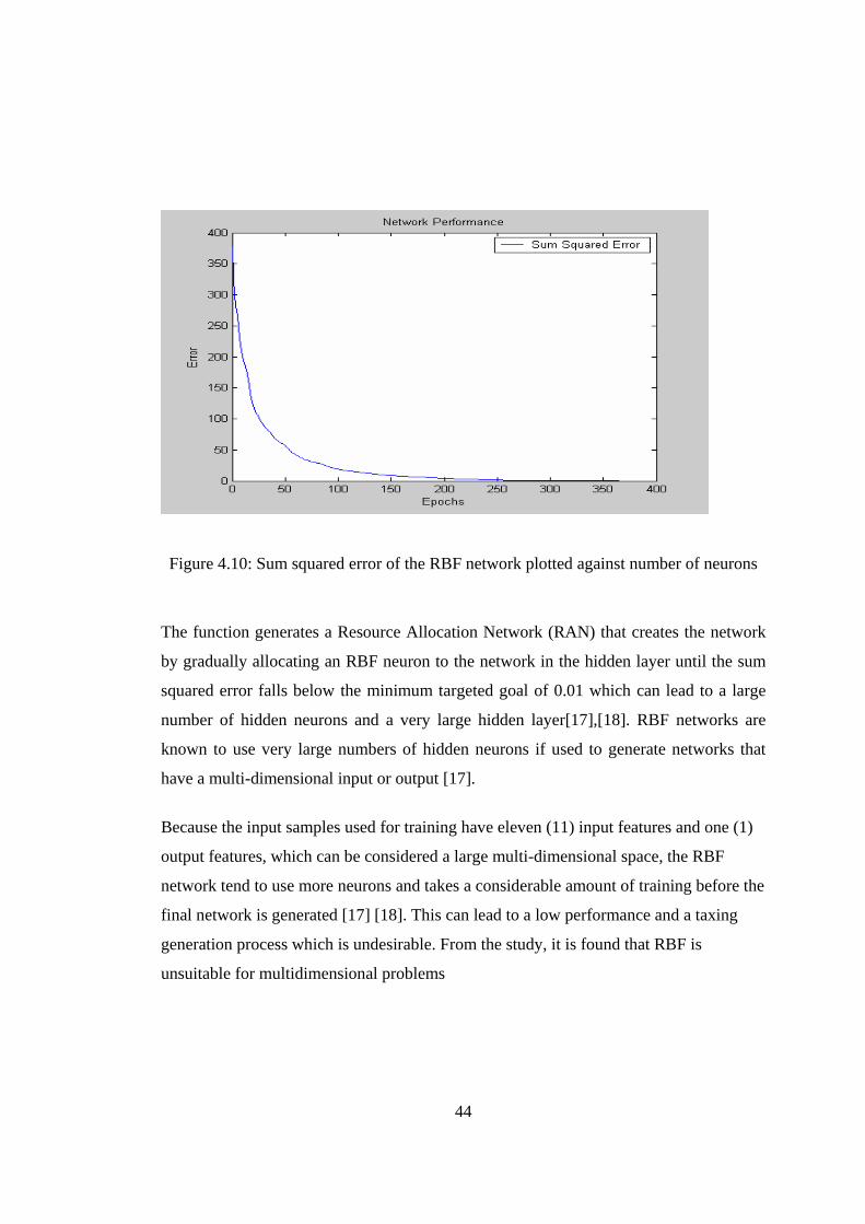
44

Figure 4.10: Sum squared error of the RBF network plotted against number of neurons

The function generates a Resource Allocation Network (RAN) that creates the network

by gradually allocating an RBF neuron to the network in the hidden layer until the sum

squared error falls below the minimum targeted goal of 0.01 which can lead to a large

number of hidden neurons and a very large hidden layer[17],[18]. RBF networks are

known to use very large numbers of hidden neurons if used to generate networks that

have a multi-dimensional input or output [17].

Because the input samples used for training have eleven (11) input features and one (1)

output features, which can be considered a large multi-dimensional space, the RBF

network tend to use more neurons and takes a considerable amount of training before the

final network is generated [17] [18]. This can lead to a low performance and a taxing

generation process which is undesirable. From the study, it is found that RBF is

unsuitable for multidimensional problems

45

4.8 Summary

This chapter describes the processes involved in utilizing ANN to predict the rice yield

data. It then present the parameters and the architecture of the ANN. It is then followed

by the behavior of data conversion algorithm using back propagation as the evaluation

method. This chapter also determine the performance of other enhance back propagation

algorithm like Quick Propagation, Conjugate Gradient, Lavenberg-Marquart and

Gradient Descent with Momentum and Adaptive Learning. It finally evaluate the

performance of RBF ANN.

Next chapter contain a description of IDSS Architecture and Prototype.

56

CHAPTER 6

CONCLUSION AND RECOMMENDATION

6.1 Conclusion

Rice is the world’s most important food crop and a primary source of food for more

than half of the world’s population [5]. Almost 90% of rice is produced and

consumed in Asia, and 96% in developing countries [6]. In Malaysia, the Third

Agriculture Policy (1998-2010) was established to meet at least 70% of Malaysia’s

demand a 5% increase over the targeted 65%. The remaining 30% comes from

imported rice mainly from Thailand, Vietnam and China [7]. Raising level of

national rice self-sufficiency has become a strategic issue in the agricultural ministry

of Malaysia. The numerous problem associated with rice farming include monitoring

the status of nutrient soil, maintaining irrigation infrastructures, obtaining quality

seedlings, controlling pests, weeds and diseases, and many other problems that need

to be addressed in order to increase productivity [8]. These problems can be

overcome with a good prediction system that can predict rice yield given the input

parameters.

This study has successfully investigated the above-mentioned problem and has

produced an intelligent decision support system (IDSS) that can predict rice yield. In

view of the objective outlined in Chapter 1, the study has produced valuable findings

as follows;

57

(a) Identification of the format and values for input parameters

affecting the rice yield

(b) Development of data conversion algorithm for input parameters

affecting rice yield.

(c) Development of a suitable ANN Model as an intelligent component in

the IDSS.

(d) Construction of the IDSS architecture to predict rice yield.

(e) Development of a web-based IDSS prototype.

The IDSS known as IndiCA can be viewed at wwwis.fsksm.utm.my/indica

6.2 Recommendation

As follows are the recommendations proposed in order to enhance the prototype;

• The IDSS that has been successfully developed is only a part of precision

farming technologies for rice. In order to make it complete other

technologies must be included such as global positioning system and

geographical information system.

• The IDSS architecture is generic hence it can be utilized to develop the IDSS

prototype for other types of crop/plants like oil palm, grape, ‘harum manis’

mango, maize, sugar cane and alike.

• Efforts should be made to transform the prototype into a fully used decision

support system through the commercialization of research findings.

REFERENCES [1] Rains, G.C., and Thomas, D.L., “Precision Farming: An Introduction”, The

cooperative extension service, The University of Georgia College of Agricultural and Environmental Sciences, Bulletin 1186, 2002 from http://www.ces.uga.edu/pubcd/b1186.htm.

[2] Winder, J. and Goddard, T., “About Precision Farming”, Agriculture, Food and Rural Development, Government of Alberta, 2001, from http://www1.agric.gov.ab.ca/$department/deptdocs.nsf/all/sag1950.

[3] Safa, B., Khalili, A., Teshnehlab, M. and Liaghat, A., “Prediction of Wheat Yield Using Artificial Neural Networks”, in 25th Conf. on Agricultural and Forest Meteorology, 2002.

[4] Lowenberg-DeBoer, J, Economics of Precision Farming: Payoff in the Future, http://pasture.ecn.purdue.edu/~mmorgan/PFI/pfiecon.html - 1/4/2002

[5] Khush, G.S., “Harnessing Science and Technology For Sustainable Rice Based Production Systems”, Conf. on Food and Agricultural Organization Rice Conference, 2004.

[6] Hossain, M. and Narciso, J., “Global Rice Economy: Long Term Perspectives”, Conf. on Food and Agricultural Organization Rice Conference, 2004.

[7] Loh, F. F., “Future of Padi in The Balance”, The Star May 21, 2001, retrieved March 21, 2004, from Koleksi Keratan Akhbar Perputakaan Sultanah Bahiyah UUM.

[8] MARDI, “Manual Penanaman Padi Berhasil Tinggi Edisi 1/2001”, Malaysian Agriculture research and Development Institute. Malaysian Ministry of Agriculture, 2002.

[9] Sudduth, K., Fraisse, C., Drummond, S. and Kitchen, N., “Analysis of Spatial Factors Influencing Crop Yield”, in Proc. Of Int. Conf. on Precision Agriculture, pp. 129-140, 1996.

[11] Liu, J., Goering, C.E. and Tian, L., “A Neural Network for Setting Target Corn Yields”, transaction of the ASAE. Vol. 44(3): 705-713, 2001.

[12] O’Neal, M.R., Engel, B.A., Ess, D.R. and Frankenberger, J.R., “Neural Network Prediction Of Maize Yield Using Alternative Data Coding Algorithms”, Biosystems Engineering 83(1), pp: 31-45, 2002.

[13] Turban, E.,” Decision Support System and Expert Systems “, Prentice Hall, pp: 694, 1998.

[14] Mendelsohn. Lou., “Preprocessing data for neural network”, Stock Market Technologies. [15] Karayiannis, Nicolaos B., Randolph-Gips, Mary M., “On The Construction and Training of Reformulated Radial Basis Function Neural Networks”, IEEE Transactions on Neural Networks, Vol. 14, July 2003. [16] Carse, B., et. al., “Evolving Radial Basis Function Neural Networks using a

Genetic Algorithm”, IEEE International Conference on Evolutionary Computation 1995, Vol. 1, pg. 300, December 1995.

[17] K. Na Nakornphanom, Lursinsap, C., Rugchatjaroen, A., “Fault Immunization Model for Elliptic Radial Basis Function Neuron”, Proceedings of the 9th

International Conference on Neural Information Processing 2002 (ICONIP’02), Vol.2, November 2002.

[18] Sundararajan, N., Saratchandran, P. and Lu, Y. W., “Radial Basis Function Neural Networks with Sequential Learning: MRAN and Its Applications”, 1st ed. Singapore: World Scientific, 1999.

[19] Alldrin, N., Smith, A. and Trunbull, D., “Classifying Facial Expression with Radial Basis Function Networks using Gradient Descent and K-Means”, Department of Computer Science, University of California, San Diego, 2003, from http://www.cs.ucsd.edu/~dturnbul/Papers/RBFproject.pdf.

[20] Documentation for MathWorks Products, Release 14, from http://www.mathworks.com/access/helpdesk/help/toolbox/nnet/linfilt6.html

[21] Ministry of Agriculture and Agro-based Industry, 2004. MOA Incorporated Homepage. Downloaded from http://agrolink.moa.my/.

[22] Aggarwal, P. K. and Penning de Vries, F. W. T., “Potential and water limited wheat yield in rice-based cropping systems in southeast Asia,”. Agric. Syst. 30: 49–69, 1989.

[23] Drummond, S.T et al, Predictive Ability of Neural Networks for Site-Specific Yield Estimation, Second International Geospatila Information in Agriculture and Forestry Conference, Lake Buena Visat, Florida, 10-12th Jan 2000

[24] S.Haykin. (1999). Neural networks: a comprehensive foundation. 2nd Edn. Englewood Cliffs, NJ:Prentice-Hall.

[25] Puteh Saad. (2003). Trademark image classification approaches using neural network and rough set theory. Ph.D. Dissertation, University Technology Malaysia

[26] Tsoukalas, L. H. and Uhrig, R. E. (1997). Fuzzy and neural approaches in engineering. John Wiley & Sons Inc., New York, USA.

[27] LeCun, Y. (1993). Efficient learning and second-order methods. A Tutorial at NIPS 93, Denver, USA.

[28] Bigus, J. P. (1996). Data mining with neural networks: solving business problems from application development to decision support. McGraw-Hill Co., Inc., New York, USA.

[29] W.A.Ahmad. (2002). Data preprocessing for neural nets. Proc. of the Int. Conf. on Artificial Intelligence in Engineering & Technology (ICAiET).pp.683-686.

[30] Puteh Saad, M Rizon M Juhari, Nor Khairah Jamaludin, Siti Sakira Kamarudin, Aryati Bakri and Nursalasawati Rusli(2004), Backpropagation Algorithm for Rice Yield Prediction, Proc. of the Ninth Int. Symp. on Artificial Life and Robotics (AROB 9th ’04) Beppu, Oita, Japan.

A. Project Identification

1. Project number : :04-02-06-0066 EA 001

2. Project title : Development of Intelligent Decision Support System for Rice

Yield Prediction in Precision Farming

3. Project Leader : Assoc. Prof. Dr. Puteh binti Saad

B. Type of research

Indicate the type of research of the project (Please see definitions in the Guidelines for

completing the Application Form)

Scientific research (fundamental research)

⁄ Technology development (applied research)

Product/process development (design and engineering)

Social/policy research

C. Objectives of the project

1. Socio-economic objectives

Which socio-economic objectives are addressed by the project? (Please identify

the sector, SEO Category and SEO Group under which the project falls. Refer the

Malaysian R&D Classification System brochure for SEO Group code) Sector : Services & IT (04)

SEO Category : Information and Communication Services (S20900)

SEO Group and Code : Computer Software and Services (S20901)

2. Fields of research

Which are the two main FOR Categories, FOR Group, and FOR Areas of your

project? (Please refer to the Malaysia R&D Classification System brochure for the

FOR Group Code)

a. Primary field of research

FOR Category : Information, Computers and Communication Tech. (F10500)

FOR Group and Code : F10501 Information System

FOR Area : Artificial Intelligence (AI)

BENEFIT REPORT I. Description of the Project

b. Secondary field of research

FOR Category: F10900 Agricultural Sciences

FOR Group and Code: F10902 Crop and Pasture Production (including rice) FOR Area: Agronomy

D. Project duration

What was the duration of the project?

Three (3) years

E. Project manpower

How many man-months did the project involve?

Forty nine (49) man-months

F. Project costs

What were the total project expenses of the project

RM134,700.00

G. Project funding

Which were the funding sources for the project?

Funding sources Total Allocation (RM)

___IRPA________ _____134,700.00______

______________________ _________________________

II. Direct Output of the Project

A. Technical contribution of the project

1. What was the achieved direct output of the project:

For scientific (fundamental) research projects?

Algorithm

Structure

Data

Other, Please specify:

_______________________________________________

For technology development (applied research) project:

Method/technique

Demonstrator/prototype


_______________________________________________

For product/process development (design and engineering) projects:

Product/component

Process

Software


_______________________________________________

2. How would you characterize the quality of this output?

Significant breakthrough

Major improvement

Minor improvement

/

/

/

/

/

B. Contribution of the project knowledge

1. How has the output of the project been documented?

Detailed project report

Product/process specification documents

Other, please specify:

Prototype

2. Did the project create an intellectual property stock?

Patent obtained

Patent pending

Patent application will be filed

Copyright

3. What publications are available?

Articles (s) in scientific publications How many:2

Papers (s) delivered at conferences/seminars How many: 6

Book


Thesis 1, Project Report 1

4. How significant are citations of the results?

Citations in national publications How many:

Citations in international publications How many:

Not Yet

Not known

/

/

/

/

/

/

III. Organizational Outcomes of the Project

A. Contribution of the project to expertise development

1. How did the project contribute to expertise?

PhD degrees How many:

MSc degrees How many: 1

Research staff with new specialty How many:

Other, Please specify: ________________________________________________

2. How significant is this expertise?

One of the key areas of priority for Malaysia

An important area, but not a priority one

B. Economic contribution of the project?

1. How has the economic contribution of the project materialized?

Sales of manufactured product/equipment

Royalties from licensing

Cost saving

Time saving

Other, Please specify: _________________________________________________

2. How important is this economic contribution?

High economic contribution Value : RM

Medium economic contribution Value : RM50,000

Low economic contribution Value : RM

3. How important is this economic contribution?

Already materialized

Within months of project completion

Within three years of project completion

Expected in three of project completion

Unknown

/

/

/

/

/

/

C. Infrastructural contribution of the project

1. What infrastructural contribution has the project had?

New equipment Value : RM

New/improved facility Investment : RM

New information networks

Other, Please specify: _________________________________________________

2. How significant is this infrastructural contribution for the organization?

Not significant/does not leverage other projects

Moderately significant

Very significant/significantly leverages other projects

D. Contribution of the project to the organization’s reputation

1. How has the project contributed to increasing the reputation of the

organization

Recognition as a Centre of Excellence

National award

International award

Demand for advisory services

Invitations to give speeches on conferences

Visits from other organization

Other, Please specify: Enable to apply for another e-science grant for similar project

2. How important is the project’s contribution to the organization’s

reputation?

Not significant

Moderately significant

Very significant

/

/

/

IV. National Impacts of the Project

A. Contribution of the project to organizational linkages

1. Which kinds of linkages did the project create?

Domestic industry linkages

International industry linkages

Linkages with domestic research institutions, universities

Linkages with international research institutions, universities

2. What is the nature of the linkages

Staff exchanges

Inter-organizational project team

Research contract with a commercial client

Informal consultation


B. Social-economic contribution of the project

1. Who are the direct customer/beneficiaries of the project output?

Customers/beneficiaries: Number:

1. Kementerian Pertanian– setting agricultural policy in national planning

2. MADA – natural resources use management especially in the water use efficiency since rice is the major consumers of our national water

3. MARDI – support R&D activities especially in the area of precision farming.

4. LPP – offer advise to padi farmers to produce better quality cereals/rice with less damages to the environment and better utilization of water

5. private sectors ( can help them to wisely utilize the available resources with minimization risk to the environment)

/

/

/

2. Who has/will the socio-economic contribution of the project materialized?

Improvements in health

Improvements in safety

Improvements in the environment

Improvements in the energy consumption

Improvements in the international relations


Improve in provision of IS services

3. How important is this socio-economic contribution?

High social contribution

Medium social contribution

Low social contribution

4. When has/will this social contribution materialized?

Already materialized

Within three years of project completion

Expected in three years or more

Unknown

Date: Signature:

/

/

/

End of Project Report Guidelines A. Purpose The purpose of the End of Project is to allow the IRPA Panels and their supporting group of experts to assess the results of research projects and the technology transfer actions to be taken. B. Information Required The following Information is required in the End of Project Report : • Project summary for the Annual MPKSN Report;

• Extent of achievement of the original project objectives;

• Technology transfer and commercialization approach;

• Benefits of the project, particularly project outputs and organisational outcomes; and

• Assessment of the project team, research approach, project schedule and project

costs.

C. Responsibility The End of Project Report should be completed by the Project Leader of the IRPA-funded project. D. Timing The End of Project Report should be submitted within three months of the completion of the research project. E. Submission Procedure One copy of the End of Project is to be mailed to :

IRPA Secretariat Ministry of Science, Technology and the Environment 14th Floor, Wisma Sime Darby Jalan Raja Laut 55662 Kuala Lumpur

End of Project Report

A. Project number :04-02-06-0066 EA 001 (Vot. No.74133)

Project title: Development of Intelligent Decision Support System for Rice Yield Prediction in Precision Farming Project leader: Assoc. Prof. Dr. Puteh Binti Saad

Tel: 07-5532428 Fax: 07-556 5044

B. Summary for the MPKSN Report (for publication in the Annual MPKSN Report, please summarise project objectives, significant results achieved the, research approach and team structure) Project Objectives:

1. To investigate, design and develop data conversion and reduction algorithm for input parameters affecting rice yield.

2. To design and develop the architecture to predict crop yield given the input parameters. 3. To design and develop an intelligent decision support system for rice yield prediction.

Significant Results Achieved: Publications:

1. Puteh Saad, Siti Sakira Kamarudin, Aryati Bakri, Nor Khairah Jamaludin, Nursalasawati Rusli Rice Yield Classification using Back Propagation Algorithm, Journal of ICT 3(1). pp 67-81, Jun 2004.

2. Puteh Saad, M Rizon M Juhari, Nor Khairah Jamaludin, Siti Sakira Kamarudin, Aryati Bakri and Nursalasawati Rusli, Backpropagation Algorithm for Rice Yield Prediction, Proc. of the Ninth Int. Symp. on Artificial Life and Robotics (AROB 9th ’04) Beppu, Oita, Japan, 28-30 January 2004.

3. Siti Sakira Kamarudin, Puteh Saad, Noraslina Abdul Rahaman and Aryati Bakri, The Architecture of an Intelligent Decision Support System for Rice Yield Prediction, Proceedings of the 1st International Conference on Informatics 29-30th July 2004, pp 153-163.

4. Shahrul Nizam Yaakob, Puteh Saad and Abu Hassan Abdullah, Insect Recognition Using FuzzyARTMAP, Proc. of Int. Conf. on Robotic Vision, Information and Signal Processing (ROVISP2005), USM, 20-22th July 2005, pp 679-683.

5. Siti Sakira Kamarudin, Rajini Devi Muniandy, Puteh Saad and Aryati Bakri, Alatan Bantuan Perosak Padi untuk Petani, Proceeding of the Seminar Kebangsaan Sosio-Ekonomi & IT Ke-2 on 11-12th August 2004.

6. Puteh Saad, Shahrul Nizam Yaakob, Nurulisma Ismail, S Niza Mohammad Bajuri, Noraslina Abd Rahaman, Shuhaizar Daud, Aryati Bakri and Siti Sakira Kamarudin, Effect of Normalization on Rice Yield Prediction, 1st National Postgraduate Colloquium (NAPCOL 2004), School of Chemical Engineering, USM on 8-9 Dec 2004.

7. Puteh Saad, Nor Khairah Jamaludin, Nursalasawati Rusli, Aryati Bakri and Siti Sakira Kamarudin, Rice Yield Prediction – A Comparison between Enhanced Back Propagation Learning Algorithms, Jurnal Teknologi Maklumat, FSKSM, Jld 16. Bil 1. pp. 27-34.

8. Puteh Saad, Shahrul Nizam Yaakob, Noraslina Abdul Rahaman and Shuhaizar Daud, Aryati Bakri, Siti Sakira Kamarudin and Nurul Isma Ismail, Artificial Neural Network Modelling of Rice Yield Prediction in Precision Farming, Proceeding of the 2nd National Conf. on Computer Graphics and Multimedia, CoGRAMM04, 8-9th December 2004.

9. Puteh Saad, Shahrul Nizam Yaakob, Aryati Bakri, Siti Sakira Kamarudin, Mahmad Nor Jaafar, Noraslina Abd Rahaman and Shuhaizar Daud, Dimensionality Reduction Using Principal Component Analysis for Rice Yield Prediction, Proc. of Int. Conf. on Robotic, Vision, Information and Signal Processing (ROVISP2005), USM, 20-22 th July 2005, pp 790-794.

Prototype: The IDSS prototype has been developed and upload on a web at: http://www.is.fsksm.utm.my/indica

Research Approach We have come up with an intelligent decision support system (INdica) for rice yield prediction in the area precision farming. The components of IDSS consist of Neural Network Model, Transformation Module and Web Development Module. In order to create the Neural Network Model there are nine (9) steps involved. In Step 1 the data to be used for training and testing of the network are collected. In Step 2 training data must identified, and plan must be made for testing the performance of the network. In Step 3 and 4 a network architecture and a learning method are selected. In Step 5 is initialization of the network to the work weights and parameters, follow by modification and of the parameters as performance feedback is received. The next procedure, Step 6, is transformed the application data input into the type and format required by neural network. In Step 7 and Step 8, training and testing are conducted as an interactive process of presenting input and desired output data to the network. At Step 9 in the process, a stable set of weights is obtained. Now the network can reproduce the desired output given inputs like those in the training set. When both of them have been developed, the network will be integrated with the decision support system as an intelligent component that will be used by farmers or farm managers to predict the rice yield. The transformation model consists of decision support system and farming database. Farming database is a knowledge base to store process and transfer agricultural crops and management information obtained from farmers. The structured collection of information is stored as a database. The parameters that affect rice yield are eleven (11) default variables. The system also contain the interfaces that help farmers or farm managers to input data, view the output that generated by intelligent component and the what if scenarios. So, from this the user can have the decision in getting the maximum rice and increase the rice yield in terms quality and quantity with minimum effects to the environment. The IDSS can also be implemented on the internet through a WWW server so the user will be able to utilize the model directly via a web browser. Upgrades are immediately made available on the WWW server. The website is the centre of activity in developing operative decision support system. The web component of the IDSS of rice yield prediction is developed using PHP. The database is developed using MySQL.

Team Structure Project Leader: Assoc. Prof. Dr. Puteh binti Saad (UTM) Researchers: Aryati Bakri (UTM) Siti Sakira Kamarudin (UUM) Dr. Mahmad Nor Jaafar (MARDI) MSc Students: Shahrul Nizam Yaakob

C. Objectives achievement

• Original project objectives (Please state the specific project objectives as described in Section ll of the Application Form)

1. To investigate, design and develop data conversion and reduction algorithm for input parameters affecting rice yield.

2. To design and develop the architecture to predict crop yield given the input parameters.

3. To design and develop an intelligent decision support system for rice yield prediction

• Objectives Achieved (Please state the extent to which the project objectives were achieved) All the objectives are achieved • Objectives not achieved (Please identify the objectives that were not achieved and give reasons)

-NONE-

D. Technology Transfer/Commercialisation Approach (Please describe the approach planned to transfer/commercialise the results of the project)

This system later on will be made available as an open source application and open access through MYREN as a component of cyber farming in Malaysia. The market will be a long term benefit to the farmers and related government sectors.

E. Benefits of the Project (Please identify the actual benefits arising from the project as defined in Section lll of the Application Form. For examples of outputs, organisational outcomes and sectoral/national impacts, please refer to Section lll of the Guidelines for the Application of R&D Funding under IRPA)

• Outputs of the project and potential beneficiaries (Please describe as specifically as possible

the outputs achieved and provide an assessment of their significance to users)

The output from this project is the IDSS prototype that can be used by the following agencies: 1. Kementerian Pertanian– setting agricultural policy in national planning 2. MADA – natural resources use management especially in the water use efficiency since rice

is the major consumers of our national water 3. MARDI – support R&D activities especially in the area of precision farming. 4. LPP – offer advise to padi farmers to produce better quality cereals/rice with less damages to

the environment and better utilization of water private sectors ( can help them to wisely utilize the available resources with minimization risk to the environment)

• Organisational Outcomes (Please describe as specifically as possible the organisational benefits arising from the project and provide an assessment of their significance)

1. Publications in terms of Journal papers and Conference Proceedings 2. Engage in high level R & D activities that meet the national objectives 3. Development of Expertise on Decision Support System Component in Precision Farming 4. 1 M.Sc. Student

• National Impacts (If known at this point in time, please describes specifically as possible the potential

sectoral/national benefits arising from the project and provide an assessment of their significance)

1. Increase quantity and quality of national rice production 2. Increase the income for rice farmers 3. Eradicate poverty 4. Export rice outside Malaysia

F. Assessment of project structure

• Project Team (Please provide an assessment of how the project team performed and highlight any significant departures from plan in either structure or actual man-days utilised)

Each of the project member perform their tasks accordingly, although they are geographically separated

• Collaborations (Please describe the nature of collaborations with other research organisations and/or

industry)

G. Assessment of Research Approach (Please highlight the main steps actually performed and indicate any major departure from the planned approach or any major difficulty encountered) The steps are according to the planned milestones written in the IRPA application form.

H. Assessment of the Project Schedule (Please make any relevant comment regarding the actual duration

of the project and highlight any significant variation from plan) The implementation is according the schedule proposed earlier in the IRPA application form

I. Assessment of Project Costs (Please comment on the appropriateness of the original budget and highlight any major departure from the planned budget)

NONE

J. Additional Project Funding Obtained (In case of involvement of other funding sources, please indicate the source and total funding provided) NONE

K. Other Remarks (Please include any other comment which you feel is relevant for the evaluation of this

project)

This project is a part of a whole precision farming system. In order to complete the whole system other modules must be included such as data acquisition module, rice plant monitoring module, weather forecast module, automatic monitoring of water level in the rice field.

1

Lampiran 20

UTM/RMC/F/0024 (1998)

UNIVERSITI TEKNOLOGI MALAYSIA

BORANG PENGESAHAN LAPORAN AKHIR PENYELIDIKAN

TAJUK PROJEK : Development of Intelligent Decision Support System for Rice Yield Prediction in Precision Farming Saya PROF. MADYA DR. PUTEH BINTI SAAD (HURUF BESAR) Mengaku membenarkan Laporan Akhir Penyelidikan ini disimpan di Perpustakaan Universiti Teknologi Malaysia dengan syarat-syarat kegunaan seperti berikut :

1. Laporan Akhir Penyelidikan ini adalah hakmilik Universiti Teknologi Malaysia 2. Perpustakaan Universiti Teknologi Malaysia dibenarkan membuat salinan untuk tujuan rujukan sahaja. 3. Perpustakaan dibenarkan membuat penjualan salinan Laporan Akhir Penyelidikan ini bagi kategori TIDAK

TERHAD 4. * Sila tandakan ( / )

SULIT (Mengandungi maklumat yang berdarjah keselamatan atau Kepentingan Malaysia seperti yang termaktub di dalam AKTA RAHSIA RASMI 1972)

TERHAD (Mengandungi maklumat TERHAD yang telah ditentukan oleh Organisasi/badan di mana penyelidikan dijalankan)

TIDAK TERHAD ____________________________________________ TANDATANGAN KETUA PENYELIDIK ____________________________________________ Nama & Cop Ketua Penyelidik Tarikh : 10 Mach 2006

INdica INTELLIGENT DECISION SUPPORT SYSTEM FOR … · Pertanian dan Asas Tani, MADA, MARDI, LPP dan...

Documents

Transcript of INdica INTELLIGENT DECISION SUPPORT SYSTEM FOR … · Pertanian dan Asas Tani, MADA, MARDI, LPP dan...