Keefisyenan Sistem Capaian Maklumat - .: FTSM - … 3 Struktur Fail.doc · Web viewDalam jadual 1,...

BAB 3 STURKTUR FAIL

1.0 Pengenalan

Keefisyenan mengukur jangka masa keputusan dicapai [2]. Ia boleh dikira dengan

menggunakan analisis kompleksiti algoritma piawai (algorithmic complexity analysis)

atau dengan pengukuran yang lebih empirikal menggunakan statistik seperti masa

tindak balas, disk I/O, dll.

Kebanyakkan sistem capaian maklumat tertumpu kepada pengukuran

keberkesanan (effectiveness). Dengan itu, banyak pengkaji capaian maklumat lebih

memfokus kepada keberkesanan dan mengabaikan keefisyenan. Sedangkan realitinya,

kejayaan sistem komersil bergantung kepada keefisyenan [2]. Sistem yang mengambil

masa terlalu lama untuk memberikan maklum balas, selalunya tidak akan digunakan.

Terdapat hanya beberapa kaedah untuk meningkatkan keefisyenan. Kaedah

pertama melibatkan langkah pemprosesan bagi membangunkan indeks songsang.

Indeks merupakan struktur biasa bagi kesemua sistem komersil, di mana ia

mengenalpasti senarai dokumen yang mengandungi setiap katakunci yang diberikan.

Kaedah kedua pula merupakan permprosesan kueri. Sesetengah katakunci atau

perkataan mungkin diabaikan dan beberapa langkah pendek mungkin diambil

berdasarkan kepada kueri. Walaubagaimanapun, pengurangan masa pemprosesan

melibatkan ketepatan, dengan itu, pemerhatian yang teliti terhadap kesan penggunaan

teknik-teknik berkenaan perlu dilakukan.

Kaedah ketiga pula ialah fail signatur. Fail signatur menganggar satu

dokumen atau kueri menggunakan vektor-bit kecil [3]. Vektor ini boleh dibandingkan

lebih cepat daripada teks asal, tetapi ketepatan akan berkurangan.

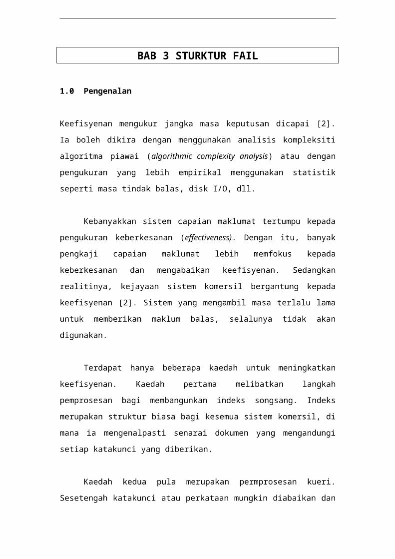
2.0 Fail Indeks Songsang

Bab 3 Struktur Fail 2

Sistem capaian maklumat membangunkan indeks songsang untuk mencari katakunci

dalam koleksi dokumen dengan berkesan[1]. Indeks songsang mengandungi dua

komponen iaitu satu senarai bagi setiap katakunci yang dipanggil indeks dan satu

senarai yang dipanggil posting list.

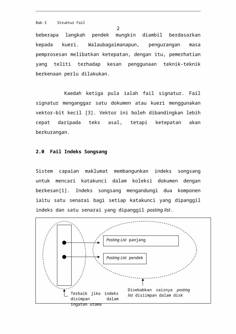
Rajah 1 : Indeks songsang

Andaikan satu koleksi dokumen di mana dokumen 1 mengandungi empat

kewujudan apple dan dua kewujudan pie. Dokumen 2 pula mengandungi tiga

kewujudan apple. Indeks akan mengandungi dua kemasukan katakunci iaitu apple dan

pie. Posting list pula merupakan senarai terpaut yang berhubung dengan setiap satu

katakunci berkenaan. Sebagai contoh,

Apple (2,3) (1,4)

Pie (1,2)

Kemasukan pada posting list disimpan dalam susunan menurun melalui

nombor dokumen kerana kemasukan pada pangkal senarai adalah lebih efisyen

berbanding pada hujung senarai. Pembinaan indeks songsang adalah mahal tetapi

dengan adanya indeks tersebut, proses kueri lebih mudah dilaksanakan.

Posting List panjang

Posting List pendek

Terbaik jika indeks disimpan dalam ingatan utama

Disebabkan saiznya posting list disiimpan dalam disk

apple

pie

32

23

1

41


Rajah 2 : Contoh Indeks Songsang

Semasa pemprosesan, posting list disimpan dalam ingatan. Ingatan

diumpukkan secara dinamik bagi setiap kemasukan baru posting list. Bagi setiap

umpukan ingatan, semakan dibuat bagi memeriksa jika ingatan yang disediakan unuk

pengindeksan telah penuh. Jika penuh, pemprosesan akan diberhentikan sementara

kesemua posting list di dalam ingatan dipindahkan ke dalam disk. Pemprosesan

diteruskan semula dengan posting list yang baru ditulis dan bagi kemasukan posting

list yang mempunyai katakunci yang sama dipautkan bersama.

Pemprosesan indeks ditamatkan apabila kesemua perkataan/katakunci telah

diproses. Pada masa ini, frekuensi dokumen songsang (idf) bagi setiap katakunci

dikira dengan melihat keseluruhan senarai katakunci yang unik. Idf mengukur

keunikan katakunci dalam koleksi. Semakin tinggi nilainya, semakin unik katakunci

tersebut. Setelah idf dikira, pemberat dokumen boleh dikira dengan melihat

keseluruhan posting list bagi setiap katakunci.

Kemasukan dalam senarai boleh juga mengandungi lokasi katakunci dalam

dokumen bagi menyediakan pencarian kesamaan. Lokasi ini boleh merujuk kepada

perkataan atau huruf. Lokasi perkataan (contoh: lokasi i merujuk kepada perkataan

ke-i) menyelesaikan kueri frasa atau kesamaan, manakala lokasi huruf (contoh: lokasi

i ialah huruf ke-i) menyediakan akses terus kepada lokasi teks yang berpadanan.

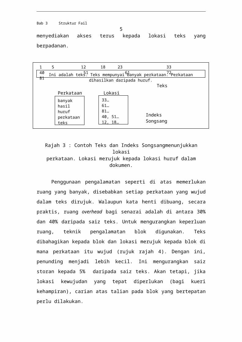
Ini adalah teks. Teks mempunyai banyak perkataan. Perkataan dihasilkan daripada huruf.

banyakhasilhuruf perkataanteks

1 5 12 18 23 33 40 51 61 72 81

33…61…81… 40, 51…12, 18…

Perkataan Lokasi

Indeks Songsang

Teks


Rajah 3 : Contoh Teks dan Indeks Songsangmenunjukkan lokasi perkataan. Lokasi merujuk kepada lokasi huruf dalam dokumen.

Penggunaan pengalamatan seperti di atas memerlukan ruang yang banyak,

disebabkan setiap perkataan yang wujud dalam teks dirujuk. Walaupun kata henti

dibuang, secara praktis, ruang overhead bagi senarai adalah di antara 30% dan 40%

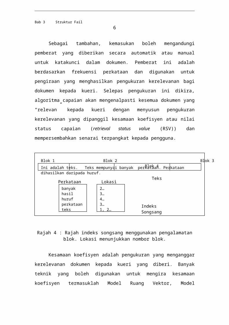
daripada saiz teks. Untuk mengurangkan keperluan ruang, teknik pengalamatan blok

digunakan. Teks dibahagikan kepada blok dan lokasi merujuk kepada blok di mana

perkataan itu wujud (rujuk rajah 4). Dengan ini, penunding menjadi lebih kecil. Ini

mengurangkan saiz storan kepada 5% daripada saiz teks. Akan tetapi, jika lokasi

kewujudan yang tepat diperlukan (bagi kueri kehampiran), carian atas talian pada blok

yang bertepatan perlu dilakukan.

Sebagai tambahan, kemasukan boleh mengandungi pemberat yang diberikan

secara automatik atau manual untuk katakunci dalam dokumen. Pemberat ini adalah

berdasarkan frekuensi perkataan dan digunakan untuk pengiraan yang menghasilkan

pengukuran kerelevanan bagi dokumen kepada kueri. Selepas pengukuran ini dikira,

algoritma capaian akan mengenalpasti kesemua dokumen yang “relevan” kepada

kueri dengan menyusun pengukuran kerelevanan yang dipanggil kesamaan koefisyen

atau nilai status capaian (retrieval status value (RSV)) dan mempersembahkan senarai

terpangkat kepada pengguna.

Rajah 4 : Rajah indeks songsang menggunakan pengalamatan blok. Lokasi menunjukkan nombor blok.

Ini adalah teks. Teks mempunyai banyak perkataan. Perkataan dihasilkan daripada huruf.

banyakhasilhuruf perkataanteks

Blok 1 Blok 2 Blok 3 Blok 4

2…3…4… 3…1, 2…

Perkataan Lokasi

Indeks Songsang

Teks


Kesamaan koefisyen adalah pengukuran yang menganggar kerelevanan

dokumen kepada kueri yang diberi. Banyak teknik yang boleh digunakan untuk

mengira kesamaan koefisyen termasuklah Model Ruang Vektor, Model

Kebarangkalian, Model Lanjutan Boolean, Algortima Genetik dan Rangkaian Neural.

Pengindeksan memerlukan overhead tambahan memandangkan keseluruhan

koleksi dilihat dan I/O yang besar diperlukan untuk menghasilkan perwakilan indeks

songsang yang efisyen bagi simpanan sekunder (secondary storage).

Walaubagaimanapun, penggunaan pengindeksan telah menunjukkan penurunan

jumlah I/O yang diperlukan untuk memenuhi kueri yang terhasil. Setelah menerima

kueri, indeks dilihat, posting list yang berkaitan dicapai dan dokumen dipangkat

berdasarkan kandungan posting list.

Kebanyakkan saiz indeks bersamaan atau melebihi saiz teks yang asal. Ini

bermakna keperluan storan barganda disebabkan oleh indeks. Akan tetapi, pemadatan

indeks menghasilkan pengurangan ruang storan kepada 10% daripada teks asal.

Katakunci yang disimpan dalam indeks bergantung kepada Parsing Algorithm yang

diamalkan atau dilaksanakan.

Saiz bagi posting list dalam indeks songsang boleh dianggarkan menggunakan

Taburan Zipfian – Zipf mencadangkan bahawa taburan frekuensi katakunci dalam

bahasa tabii ialah jika kesemua katakunci disusun dan diberi pemangkatan, produk

bagi frekuensi dan pemangkatan tersebut akan menjadi malar. Dalam jadual 1,

Taburan Zipfian digambarkan apabila pemalar adalah 1. Dengan menggunakan F=C/r,

dimana r adalah pangkat, F adalah frekuensi dan C ialah nilai pemalar, penganggaran

jumlah kewujudan katakunci yang diberi boleh dibuat. Pemalar, C, adalah spesifik-

domain dan bersamaan dengan jumlah kewujudan bagi kebanyakkan katakunci yang

kerap.

Pangkat Frekuensi Pemalar

1 1.00 1

2 0.50 1

3 0.33 1


4 0.25 1

5 0.20 1

Jadual 1 : Contoh Taburan Zipf

2.1 Struktur data yang digunakan dalam fail songsang

Struktur data yang biasa digunakan ialah:

i. pohon B

ii. pohon gelintar digital (trie)

iii. tatasusunan terisih (sorted array)

iv. Cincangan (bincang dalam bab XX)

2.1.1 Pohon-B

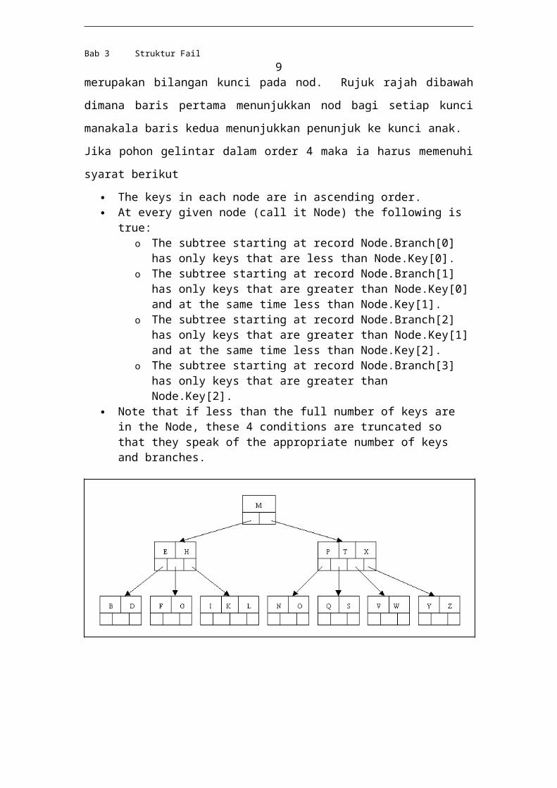
Pohon-B biasanya digunakan untuk tujuan gelintaran data. Ia mesti mempunyai

nombor kunci dan anak. Pohon pada order m nerupakan pohon dimana setiap nod

mempunyai sebanyak-banyaknya m anak. Bagi setiap nod, jika k merupakan bilangan

sebenar anak pada nod, maka k-1 merupakan bilangan kunci pada nod. Rujuk rajah

dibawah dimana baris pertama menunjukkan nod bagi setiap kunci manakala baris

kedua menunjukkan penunjuk ke kunci anak.

Jika pohon gelintar dalam order 4 maka ia harus memenuhi syarat berikut

The keys in each node are in ascending order. At every given node (call it Node) the following is true:

o The subtree starting at record Node.Branch[0] has only keys that are less than Node.Key[0].

o The subtree starting at record Node.Branch[1] has only keys that are greater than Node.Key[0] and at the same time less than Node.Key[1].

o The subtree starting at record Node.Branch[2] has only keys that are greater than Node.Key[1] and at the same time less than Node.Key[2].

o The subtree starting at record Node.Branch[3] has only keys that are greater than Node.Key[2].

Note that if less than the full number of keys are in the Node, these 4 conditions are truncated so that they speak of the appropriate number of keys and branches.


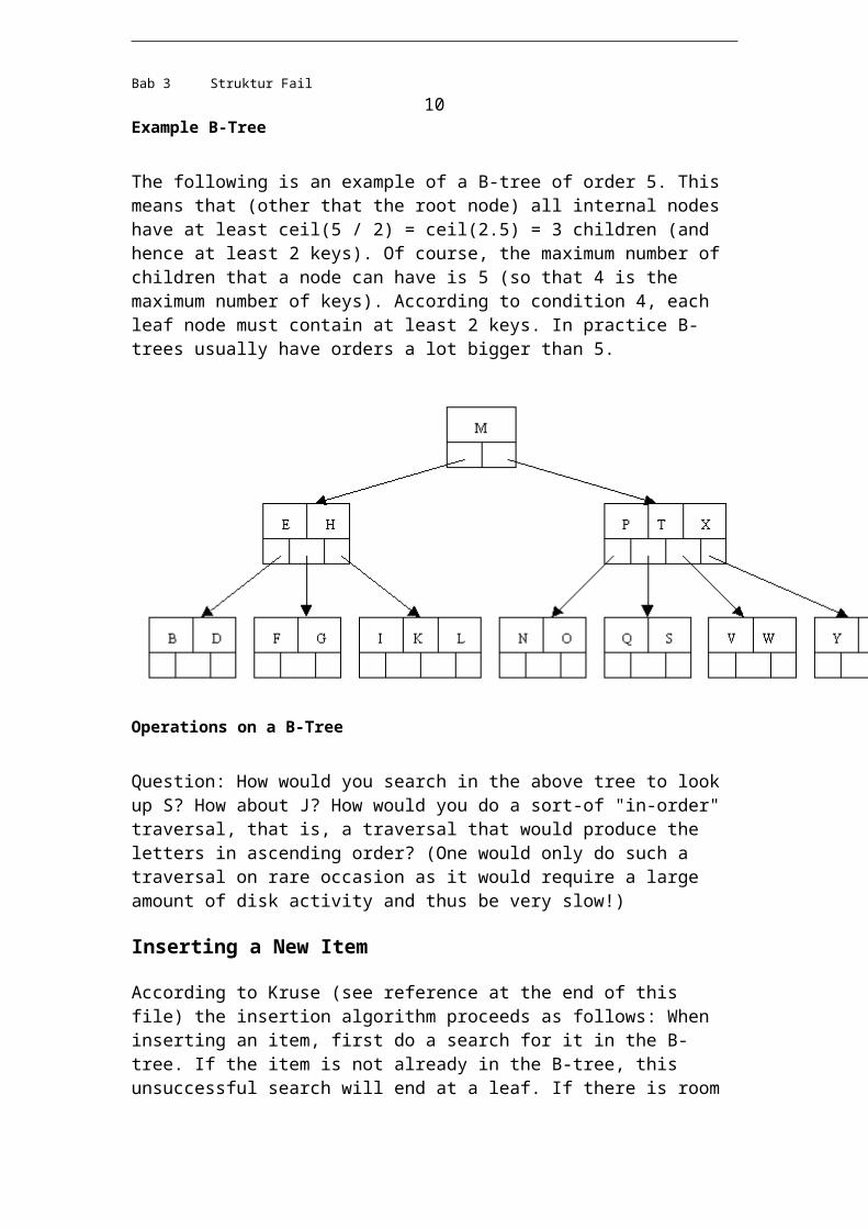
Example B-Tree

The following is an example of a B-tree of order 5. This means that (other that the root node) all internal nodes have at least ceil(5 / 2) = ceil(2.5) = 3 children (and hence at least 2 keys). Of course, the maximum number of children that a node can have is 5 (so that 4 is the maximum number of keys). According to condition 4, each leaf node must contain at least 2 keys. In practice B-trees usually have orders a lot bigger than 5.

Operations on a B-Tree

Question: How would you search in the above tree to look up S? How about J? How would you do a sort-of "in-order" traversal, that is, a traversal that would produce the letters in ascending order? (One would only do such a traversal on rare occasion as it would require a large amount of disk activity and thus be very slow!)

Inserting a New Item

According to Kruse (see reference at the end of this file) the insertion algorithm proceeds as follows: When inserting an item, first do a search for it in the B-tree. If the item is not already in the B-tree, this unsuccessful search will end at a leaf. If there is room in this leaf, just insert the new item here. Note that this may require that some existing keys be moved one to the right to make room for the new item. If instead this leaf node is full so that there is no room to add the new item, then the node must be "split" with about half of the keys going into a new node to the right of this one. The median (middle) key is moved up into the parent node. (Of course, if that node has no


room, then it may have to be split as well.) Note that when adding to an internal node, not only might we have to move some keys one position to the right, but the associated pointers have to be moved right as well. If the root node is ever split, the median key moves up into a new root node, thus causing the tree to increase in height by one.

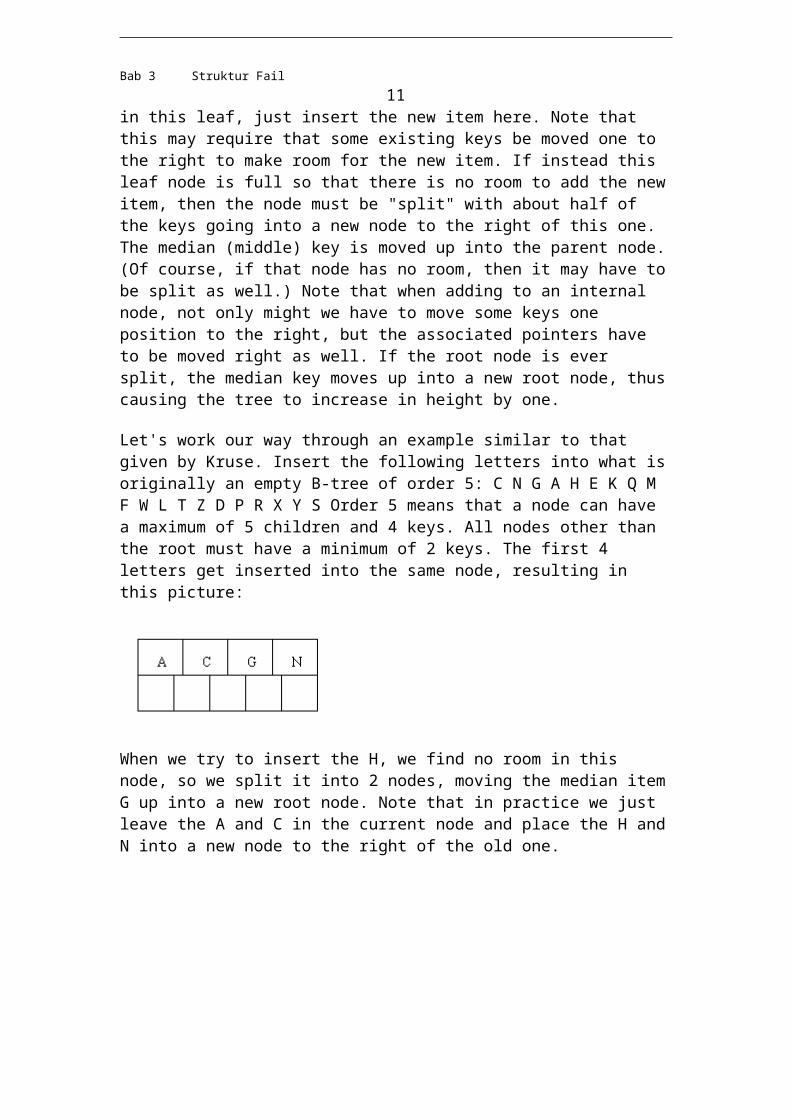
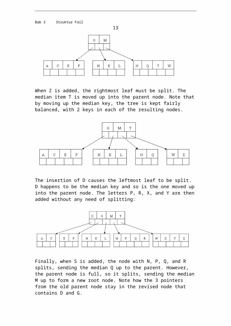
Let's work our way through an example similar to that given by Kruse. Insert the following letters into what is originally an empty B-tree of order 5: C N G A H E K Q M F W L T Z D P R X Y S Order 5 means that a node can have a maximum of 5 children and 4 keys. All nodes other than the root must have a minimum of 2 keys. The first 4 letters get inserted into the same node, resulting in this picture:

When we try to insert the H, we find no room in this node, so we split it into 2 nodes, moving the median item G up into a new root node. Note that in practice we just leave the A and C in the current node and place the H and N into a new node to the right of the old one.

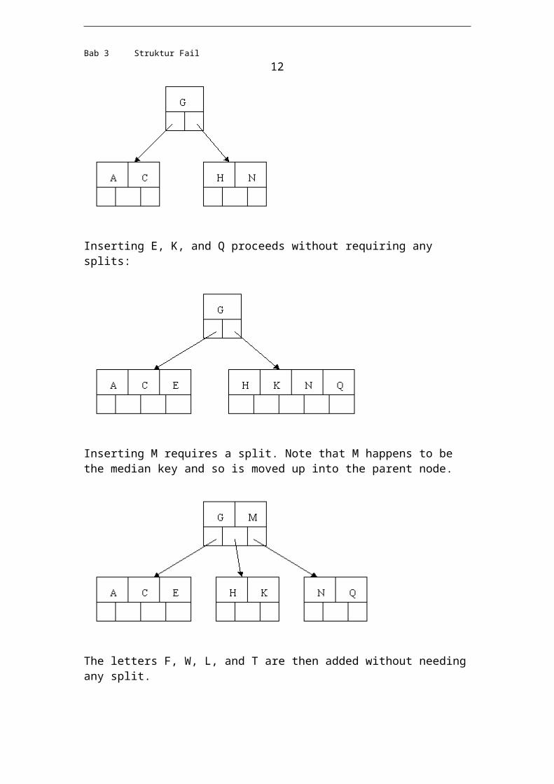
Inserting E, K, and Q proceeds without requiring any splits:


Inserting M requires a split. Note that M happens to be the median key and so is moved up into the parent node.

The letters F, W, L, and T are then added without needing any split.

When Z is added, the rightmost leaf must be split. The median item T is moved up into the parent node. Note that by moving up the median key, the tree is kept fairly balanced, with 2 keys in each of the resulting nodes.

The insertion of D causes the leftmost leaf to be split. D happens to be the median key and so is the one moved up into the parent node. The letters P, R, X, and Y are then added without any need of splitting:


Finally, when S is added, the node with N, P, Q, and R splits, sending the median Q up to the parent. However, the parent node is full, so it splits, sending the median M up to form a new root node. Note how the 3 pointers from the old parent node stay in the revised node that contains D and G.

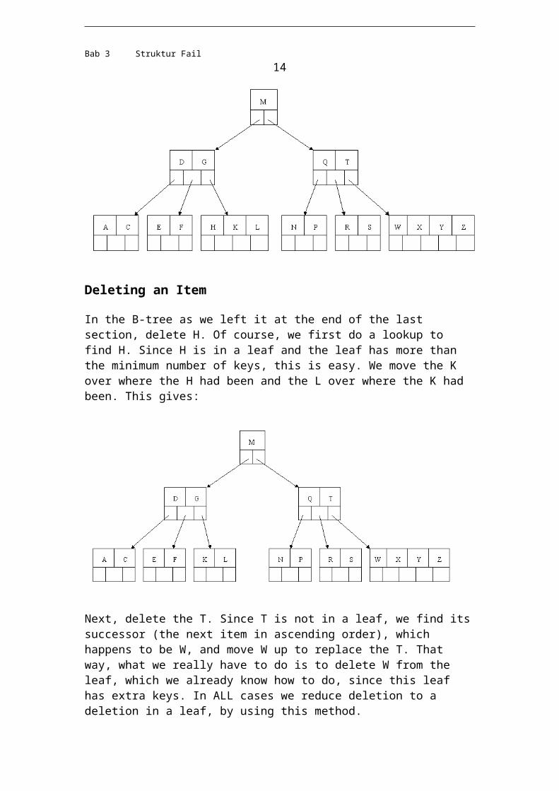
Deleting an Item

In the B-tree as we left it at the end of the last section, delete H. Of course, we first do a lookup to find H. Since H is in a leaf and the leaf has more than the minimum number of keys, this is easy. We move the K over where the H had been and the L over where the K had been. This gives:


Next, delete the T. Since T is not in a leaf, we find its successor (the next item in ascending order), which happens to be W, and move W up to replace the T. That way, what we really have to do is to delete W from the leaf, which we already know how to do, since this leaf has extra keys. In ALL cases we reduce deletion to a deletion in a leaf, by using this method.

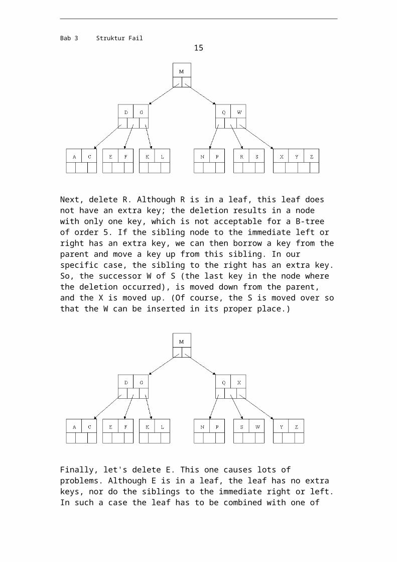
Next, delete R. Although R is in a leaf, this leaf does not have an extra key; the deletion results in a node with only one key, which is not acceptable for a B-tree of order 5. If the sibling node to the immediate left or right has an extra key, we can then borrow a key from the parent and move a key up from this sibling. In our specific case, the sibling to the right has an extra key. So, the successor W of S (the last key in the node where the deletion occurred), is moved down from the parent, and the X is moved up. (Of course, the S is moved over so that the W can be inserted in its proper place.)


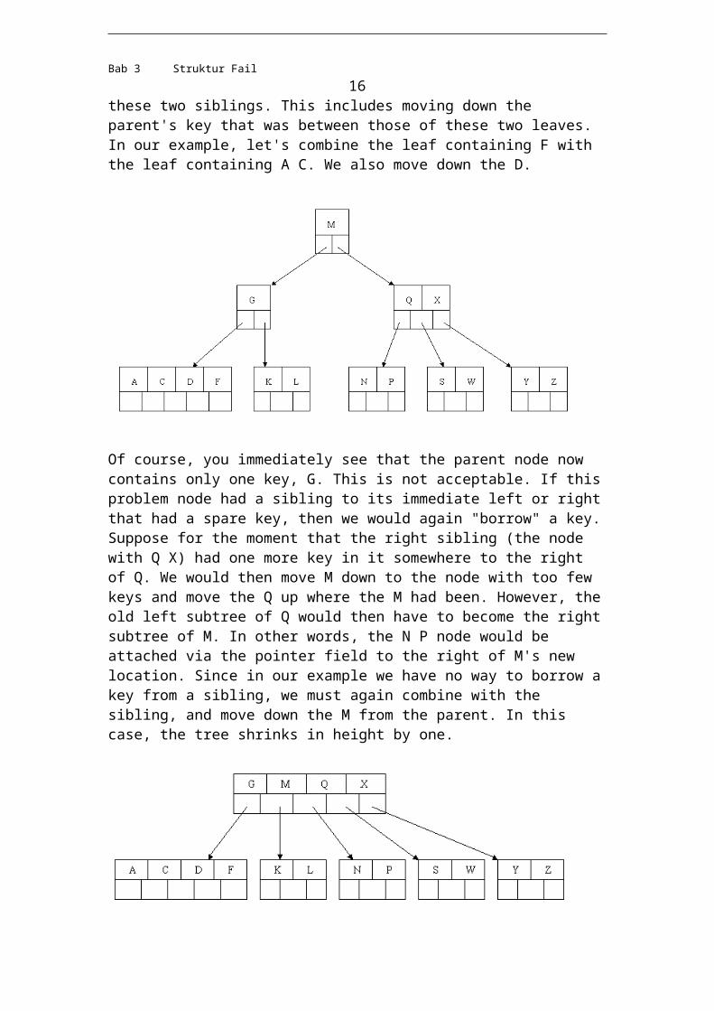
Finally, let's delete E. This one causes lots of problems. Although E is in a leaf, the leaf has no extra keys, nor do the siblings to the immediate right or left. In such a case the leaf has to be combined with one of these two siblings. This includes moving down the parent's key that was between those of these two leaves. In our example, let's combine the leaf containing F with the leaf containing A C. We also move down the D.

Of course, you immediately see that the parent node now contains only one key, G. This is not acceptable. If this problem node had a sibling to its immediate left or right that had a spare key, then we would again "borrow" a key. Suppose for the moment that the right sibling (the node with Q X) had one more key in it somewhere to the right of Q. We would then move M down to the node with too few keys and move the Q up where the M had been. However, the old left subtree of Q would then have to become the right subtree of M. In other words, the N P node would be attached via the pointer field to the right of M's new location. Since in our example we have no way to borrow a key from a sibling, we must again combine with the sibling, and move down the M from the parent. In this case, the tree shrinks in height by one.


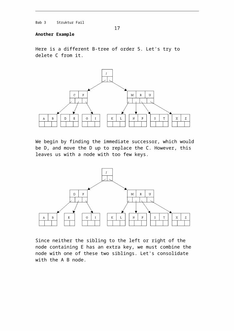
Another Example

Here is a different B-tree of order 5. Let's try to delete C from it.

We begin by finding the immediate successor, which would be D, and move the D up to replace the C. However, this leaves us with a node with too few keys.

Since neither the sibling to the left or right of the node containing E has an extra key, we must combine the node with one of these two siblings. Let's consolidate with the A B node.


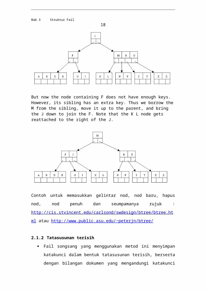
But now the node containing F does not have enough keys. However, its sibling has an extra key. Thus we borrow the M from the sibling, move it up to the parent, and bring the J down to join the F. Note that the K L node gets reattached to the right of the J.

Contoh untuk memasukkan gelintar nod, nod baru, hapus nod, nod penuh dan

seumpamanya rujuk : http://cis.stvincent.edu/carlsond/swdesign/btree/btree.html atau

http://www.public.asu.edu/~peterjn/btree/

2.1.2 Tatasusunan terisih

Fail songsang yang menggunakan metod ini menyimpan katakunci dalam

bentuk tatasusunan terisih, berserta dengan bilangan dokumen yang

mengandungi katakunci tersebut dan hubungan yang menghubungkan ke

dokumen-dokumen tersebut.

Penggelintaran dalam tatasusunan ini ialah berdasarkan penggelintaran binari.

http://www.public.asu.edu/~peterjn/btree/

http://cis.stvincent.edu/carlsond/swdesign/btree/btree.html


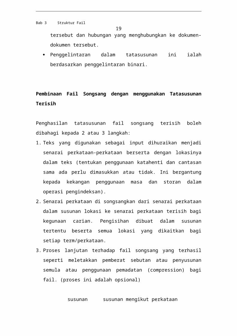
Pembinaan Fail Songsang dengan menggunakan Tatasusunan Terisih

Penghasilan tatasusunan fail songsang terisih boleh dibahagi kepada 2 atau 3 langkah:

1. Teks yang digunakan sebagai input dihuraikan menjadi senarai perkataan-

perkataan berserta dengan lokasinya dalam teks (tentukan penggunaan katahenti

dan cantasan sama ada perlu dimasukkan atau tidak. Ini bergantung kepada

kekangan penggunaan masa dan storan dalam operasi pengindeksan).

2. Senarai perkataan di songsangkan dari senarai perkataan dalam susunan lokasi ke

senarai perkataan terisih bagi kegunaan carian. Pengisihan dibuat dalam susunan

tertentu beserta semua lokasi yang dikaitkan bagi setiap term/perkataan.

3. Proses lanjutan terhadap fail songsang yang terhasil seperti meletakkan pemberat

sebutan atau penyusunan semula atau penggunaan pemadatan (compression) bagi

fail. (proses ini adalah opsional)

susunan mengikut

lokasi

susunan mengikut perkataan

hurai isih memberati

teks perkataan lokasi perkataan lokasi perkataan lokasi pemberat

Skema keseluruhan penghasilan tatasusunan fail songsang terisih

Biasanya fail songsang yang dihasilkan diproses hingga kepada format terakhir

yang lebih baik.

Oleh kerana penggelintaran dalam fail songsang biasanya berasaskan

penggelintaran binari, maka fail yang digelintar seboleh mungkin mempunyai

bilangan katakunci atau sebutan yang sedikit atau failnya yang ringkas.

Kelemahan tatasusunan terisih ialah untuk mengemaskini indeks adalah sukar, namun

kebaikannya ialah mudah dilaksanakan dan cepat.


Contoh dalam langkah pembangunan senarai terisih

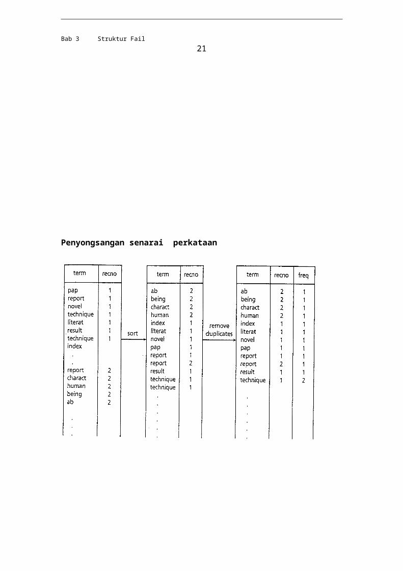
Penyongsangan senarai perkataan


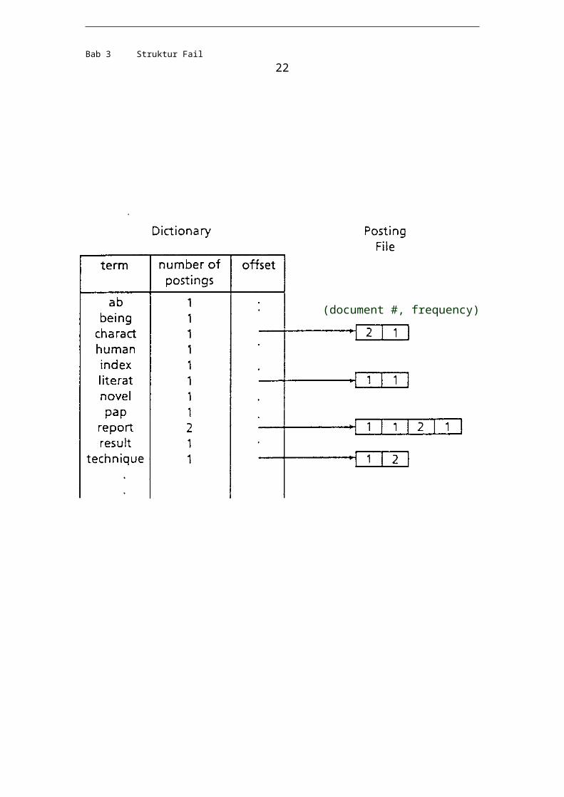
(document #, frequency)


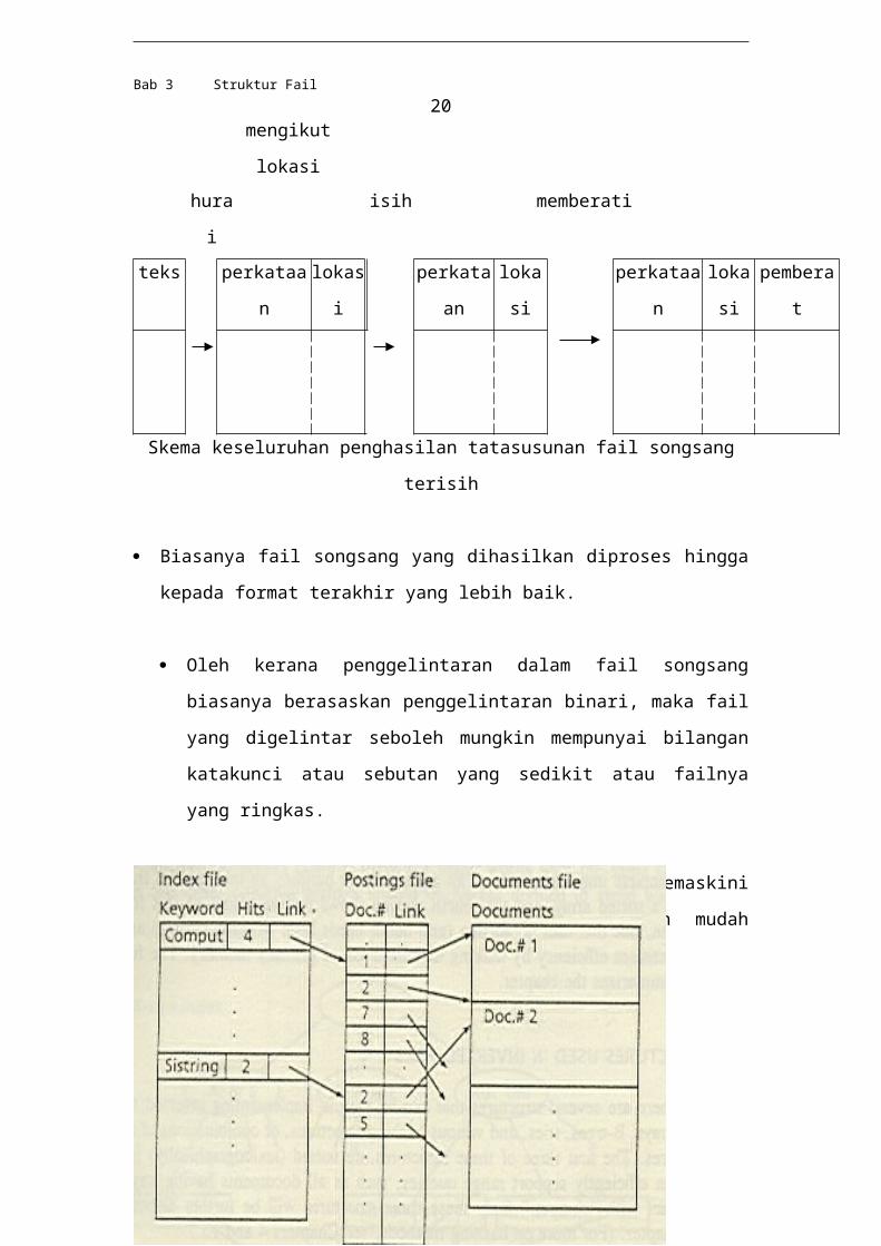
3.0 Jadual Cincangan (Hashing Table)http://cis.stvincent.edu/carlsond/swdesign/hash/hash.html

What is a Table?

A hash table is one way to create a table (sometimes called a dictionary). Typical operations are Empty, Insert, and Retrieve. The idea is that a table is a place to store data records, each containing a key value as well as other data fields (or field), so as to easily retrieve the data later by supplying a key value. The Retrieve function supplies the entire matching record of data.

What is a Hash Table?

One way to create a table, either on disk or in main memory, is to use a hash table. The goal of a hash table is to get Theta(1) lookup time, that is, constant lookup time. Rather than having to proceed through a Theta(n) sequence of comparisons as in linear search, or a Theta(lg n) sequence of comparisons as in binary search, a hash table will usually complete a lookup after just one comparison! Sometimes, however, two comparisons (or even more) are needed. A hash table thus delivers (almost) the ideal lookup time. The trade-off is that to get this great lookup time memory space is wasted. This may well be a good trade-off, however, as memory is cheap.

The idea is that we store records of data in the hash table, which is either an array (when main memory is used), or a file (if disk space is used). Each record has a key field and an associated data field. The record is stored in a location that is based on its key. The function that produces this location for each given key is called a hash function.

Let's suppose that each key field contains an integer and the data field a string (array of characters type of string). One possible hash function is hash(key) = key % prime.

Recall that % is the mod operator that gives the remainder after integer division. The constant prime holds some prime number that is the length of the table. (For technical reasons, a prime number works better.) Perhaps we are storing our hash table in an array and use prime = 101. This means that our table can hold up to 101 records, at indices 0 through 100. If we want to insert 225 into the table we compute hash(225) as 225 % 101 = 23 and store the record containing key value 225 at index 23 in the array. Of course, if this location already contains a record, then we have a problem (called a collision). More on collisions later!

If we go to look up the record with key 225, we again calculate hash(225) and get 23. We go to index 23, check that the record at that position has key value 225, and copy that record. There it is: one comparison and we completed our lookup. The situation is even more dramatic when using a file, since disk access is so much slower and every new record that has to be read adds appreciably to the lookup time. Here the hash function values are record numbers not array indices, but it works very much the same. To look up 225, we find hash(225) = 23, read record 23 from the file, check that this record does indeed have key value 225 and we are done! Only one record had to be read!


Collisions

When inserting items into a hash table, it sometimes happens that an item to be inserted hashes to the same location as an item already in the table. (Note that some method is needed to distinguish locations in use from unused locations.) The new item typically is inserted somewhere else, though we must be sure that there is still a way (and a fairly fast way) to look up the item. Here are several ways of handling collisions:

Rehash function

A second function can be used to select a second table location for the new item. If that location is also in use, the rehash function can be applied again to generate a third location, etc. The rehash function has to be such that when we use it in the lookup process we again generate the same sequence of locations. Since the idea in a hash table is to do a lookup by only looking at one location in the table, rehashing should be minimized as much as possible. In the worst case, when the table is completely filled, one could rehash over and over until every location in the table has been tried. The running time would be horrible!

Linked list approach (separate chaining)

All items that hash to the same location can be inserted in a linked list whose front pointer is stored in the given location. If the data is on disk, the linked list can be imitated by using record numbers instead of actual pointers. On disk, the hash table file would be a file of fake pointers (record numbers). Each record number would be for a record in another file, a file of nodes, where each node has a next field containing the number of the next record in the list.

Linked list inside the table (coalesced hashing)

Here each table entry is a record containing one item that hashed to this location and a record number for another item in the table that hashed to this location, which may have the record number of another that hashed to the same spot, etc. We are again using a linked list, but this list is stored within the table, whereas in the method above the list was external to the table, which only stored the front pointer for each list. Items beyond the first may be stored in an overflow area of the table (sometimes called the cellar) so as not to take up regular table space. This is the approach that I took in the example program that goes with this section. It is recommended that the overflow area take only about 15% of the space available for the table (the regular table area and overflow area combined).

Buckets

Sometimes each location in the table is a bucket which will hold a fixed number of items, all of which hashed to this same location. This speeds up lookups because there is probably no need to go look at another location. However, a bucket could fill up so that new insertions that hash to this location will need some other collision handler, such as one of the above methods.


Example Using Linear Probing

A simple rehash function is rehash(k) = (k + 1) % prime, where prime is the prime number giving the maximum number of items in the table. This is sometimes called linear probing, since when an item hashes to a location k that is already in use, the rehash function then tells us to try k + 1, the next location (unless k + 1 would be off the end of the table, in which case the rehash function sends us back to the start of the table at index 0). The next location tried would normally be k + 2, then k + 3, etc. Trying successive locations like this is simple, but it leads to clustering problems. When several items hash to the same location they build up a cluster of items that are side-by-side in the table. Any new item that hashes to any of these locations has to be rehashed and moved to the end of the cluster. Insertions to these locations tend to be slower as do lookups of the data stored there. This is because we are getting away from our goal of checking one location and finding our data item. The number of rehashes needed should be kept as small as possible. In the worst case, a table that is full except for one location just before the cluster would require Theta(n) rehashes as successive locations are tried (with wrap-around to index 0) until that one empty location is found.

Suppose we use integer key values, prime = 5, and the following functions:

hash(key) = key % prime;

rehash(k) = (k + 1) % prime;

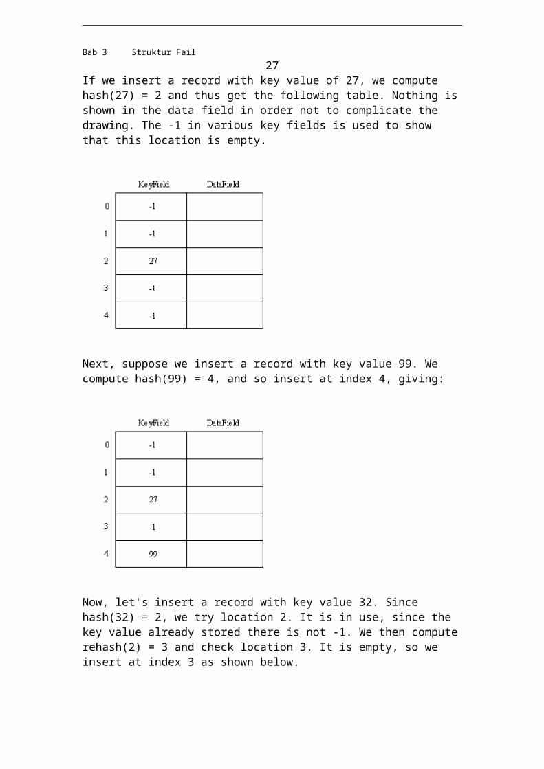
If we insert a record with key value of 27, we compute hash(27) = 2 and thus get the following table. Nothing is shown in the data field in order not to complicate the drawing. The -1 in various key fields is used to show that this location is empty.

Next, suppose we insert a record with key value 99. We compute hash(99) = 4, and so insert at index 4, giving:


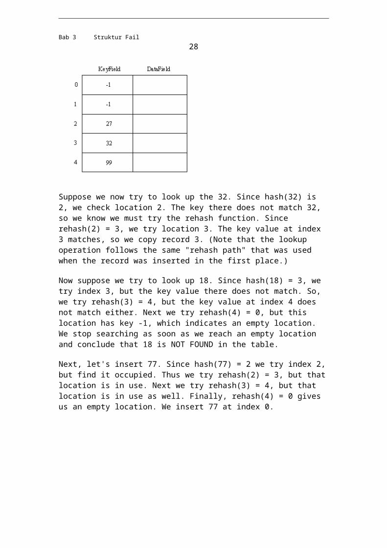
Now, let's insert a record with key value 32. Since hash(32) = 2, we try location 2. It is in use, since the key value already stored there is not -1. We then compute rehash(2) = 3 and check location 3. It is empty, so we insert at index 3 as shown below.

Suppose we now try to look up the 32. Since hash(32) is 2, we check location 2. The key there does not match 32, so we know we must try the rehash function. Since rehash(2) = 3, we try location 3. The key value at index 3 matches, so we copy record 3. (Note that the lookup operation follows the same "rehash path" that was used when the record was inserted in the first place.)

Now suppose we try to look up 18. Since hash(18) = 3, we try index 3, but the key value there does not match. So, we try rehash(3) = 4, but the key value at index 4 does not match either. Next we try rehash(4) = 0, but this location has key -1, which indicates an empty location. We stop searching as soon as we reach an empty location and conclude that 18 is NOT FOUND in the table.

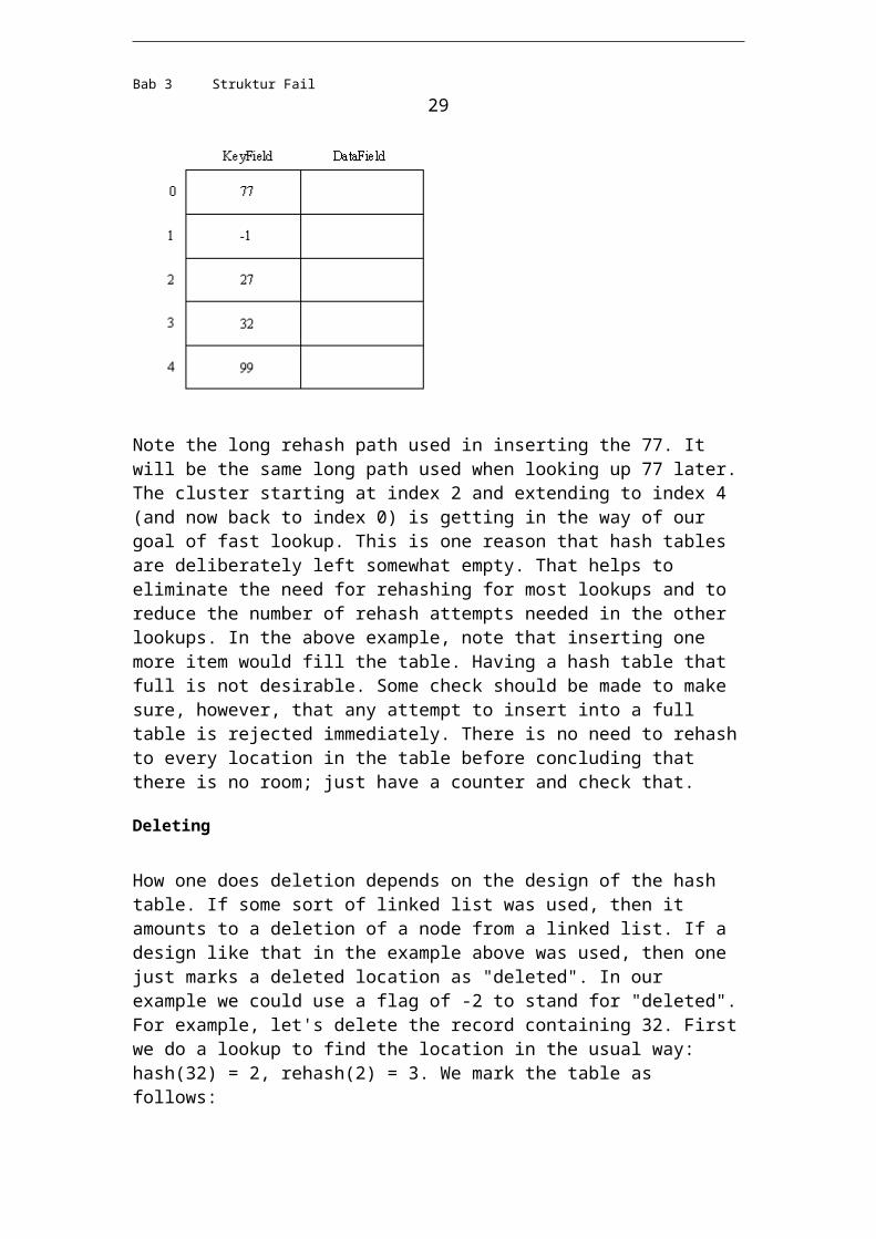
Next, let's insert 77. Since hash(77) = 2 we try index 2, but find it occupied. Thus we try rehash(2) = 3, but that location is in use. Next we try rehash(3) = 4, but that


location is in use as well. Finally, rehash(4) = 0 gives us an empty location. We insert 77 at index 0.

Note the long rehash path used in inserting the 77. It will be the same long path used when looking up 77 later. The cluster starting at index 2 and extending to index 4 (and now back to index 0) is getting in the way of our goal of fast lookup. This is one reason that hash tables are deliberately left somewhat empty. That helps to eliminate the need for rehashing for most lookups and to reduce the number of rehash attempts needed in the other lookups. In the above example, note that inserting one more item would fill the table. Having a hash table that full is not desirable. Some check should be made to make sure, however, that any attempt to insert into a full table is rejected immediately. There is no need to rehash to every location in the table before concluding that there is no room; just have a counter and check that.

Deleting

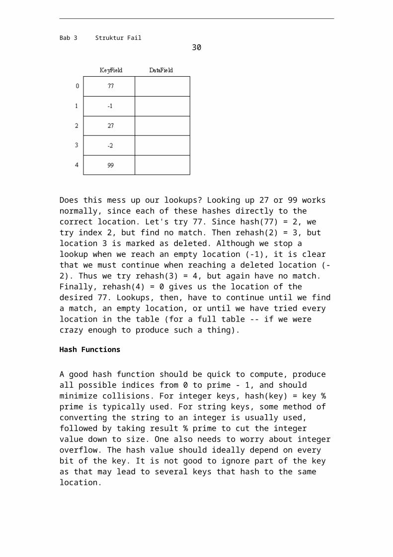
How one does deletion depends on the design of the hash table. If some sort of linked list was used, then it amounts to a deletion of a node from a linked list. If a design like that in the example above was used, then one just marks a deleted location as "deleted". In our example we could use a flag of -2 to stand for "deleted". For example, let's delete the record containing 32. First we do a lookup to find the location in the usual way: hash(32) = 2, rehash(2) = 3. We mark the table as follows:


Does this mess up our lookups? Looking up 27 or 99 works normally, since each of these hashes directly to the correct location. Let's try 77. Since hash(77) = 2, we try index 2, but find no match. Then rehash(2) = 3, but location 3 is marked as deleted. Although we stop a lookup when we reach an empty location (-1), it is clear that we must continue when reaching a deleted location (-2). Thus we try rehash(3) = 4, but again have no match. Finally, rehash(4) = 0 gives us the location of the desired 77. Lookups, then, have to continue until we find a match, an empty location, or until we have tried every location in the table (for a full table -- if we were crazy enough to produce such a thing).

Hash Functions

A good hash function should be quick to compute, produce all possible indices from 0 to prime - 1, and should minimize collisions. For integer keys, hash(key) = key % prime is typically used. For string keys, some method of converting the string to an integer is usually used, followed by taking result % prime to cut the integer value down to size. One also needs to worry about integer overflow. The hash value should ideally depend on every bit of the key. It is not good to ignore part of the key as that may lead to several keys that hash to the same location.

Here is one method for strings. Let's suppose that the strings only contain the letters of the alphabet, in upper case. In other words, we have the letters A through Z. We can translate the individual letters to the integers 0 through 25. Then we treat the string as a base 26 number. For example, CPU would be the base 26 number with digits 2, 15, 20. The decimal value of this number is 2(26^2) + 15(26) + 20. All computations are done % prime, both to avoid overflow, and because the final hash value must fit the range 0 to prime - 1. For example, if prime = 101, we would get 26^2 % 101 = 676 % 101 = 70. Then 2(26^2) % 101 = 39. The 15(26) % 101 = 390 % 101 = 87. Thus we get (39 + 87) % 101 = 126 % 101 = 25. The final hash value is thus (25 + 20) % 101 = 45. If your strings include more of the ASCII character set than this, you might want to use the ASCII value of each letter instead of mapping A to 0, B to 1, etc.

A folding method is sometimes used to hash integers. Here the key is chopped into two or more parts and the parts recombined in some easy manner. For example,


suppose the keys are 9 digit longs, such as 542981703. Chop this into 3 equal-length pieces and add them together: 542 + 981 + 703, taking the sum % prime to cut the answer down to size.

A Hash Table Example itemtype.h table.h (sets up an abstract base class for tables) hash.h (derives a hash table class) hash.cpp hash.txt (text file of data to use) hashmake.cpp (creates a hash table) hashread.cpp (reads data from a hash table)

This example uses coalesced chaining (a linked list inside the table with all items after the first in an overflow area of the table). Let's see how it works.

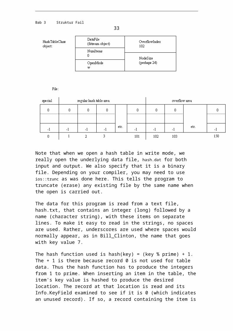
The file is organized as a binary file of records. Each record has an Info and a Next field. The Next field will contain the record number for the next record in the linked list (when we have to chain nodes together) or a -1 as a fake NULL pointer. Record 0 (the first record in the file) is not used to hold node data at all. Instead, it holds in Info.KeyField the number of items in the table. That way this count is stored permanently, along with the file. When an empty table is first created, the entire file is filled with empty nodes. Thus, the special record 0, followed by empty nodes 1 through MaxFile = 150 are written to the file. These nodes are marked as empty by placing 0 in the KeyField locations. (This assumes that 0 is not a normal KeyField value.) The regular part of the table includes nodes 1 through Prime = 101, and the overflow area is from node 102 to node MaxFile = 150. A field of the HashTableClass object, called OverflowIndex, is used to keep track of the next free record for overflow use. (Thus OverflowIndex is initially set to 102. If it reaches 151, the overflow area is full.)

The following is a drawing of a HashtableClass object, showing the five data fields. Note that the OpenMode field contains the character r or w, indicating whether the table has been opened in read or write mode. NodeSize is the number of bytes per node. Since this value is often needed, it is convenient to store it in a field of the object. The DataFile field is an fstream object containing information about the file where the table's data is held. The details of an fstream object are beyond what we will study here, but include information such as the current position in the file.

http://cis.stvincent.edu/carlsond/swdesign/hash/hashread.cpp

http://cis.stvincent.edu/carlsond/swdesign/hash/hashmake.cpp

http://cis.stvincent.edu/carlsond/swdesign/hash/hash.txt

http://cis.stvincent.edu/carlsond/swdesign/hash/hash.cpp

http://cis.stvincent.edu/carlsond/swdesign/hash/hash.h

http://cis.stvincent.edu/carlsond/swdesign/hash/table.h

http://cis.stvincent.edu/carlsond/swdesign/hash/itemtype.h


Note that when we open a hash table in write mode, we really open the underlying data file, hash.dat for both input and output. We also specify that it is a binary file. Depending on your compiler, you may need to use ios::trunc as was done here. This tells the program to truncate (erase) any existing file by the same name when the open is carried out.

The data for this program is read from a text file, hash.txt, that contains an integer (long) followed by a name (character string), with these items on separate lines. To make it easy to read in the strings, no spaces are used. Rather, underscores are used where spaces would normally appear, as in Bill_Clinton, the name that goes with key value 7.

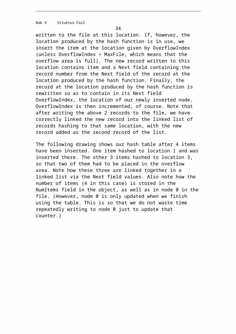
The hash function used is hash(key) = (key % prime) + 1. The + 1 is there because record 0 is not used for table data. Thus the hash function has to produce the integers from 1 to prime. When inserting an item in the table, the item's key value is hashed to produce the desired location. The record at that location is read and its Info.KeyField examined to see if it is 0 (which indicates an unused record). If so, a record containing the item is written to the file at this location. If, however, the location produced by the hash function is in use, we insert the item at the location given by OverflowIndex (unless OverflowIndex > MaxFile, which means that the overflow area is full). The new record written to this location contains item and a Next field containing the record number from the Next field of the record at the location produced by the hash function. Finally, the record at the location produced by the hash function is rewritten so as to contain in its Next field OverflowIndex, the location of our newly inserted node. OverflowIndex is then incremented, of course. Note that after writing the above 2 records to the file, we have correctly linked the new record into the linked list of records hashing to that same location, with the new record added as the second record of the list.


The following drawing shows our hash table after 4 items have been inserted. One item hashed to location 1 and was inserted there. The other 3 items hashed to location 3, so that two of them had to be placed in the overflow area. Note how these three are linked together in a linked list via the Next field values. Also note how the number of items (4 in this case) is stored in the NumItems field in the object, as well as in node 0 in the file. (However, node 0 is only updated when we finish using the table. This is so that we do not waste time repeatedly writing to node 0 just to update that counter.)

When a table is first opened for reading, the special record 0 is read in so that the number of items in the table can be discovered by examining Info.KeyField. To do a lookup of a key value, we first compute hash(key) and read in the record with that number as its location. If the key in this record matches, we are done. If not and the Next field of this record contains -1 (used as a fake NULL pointer), then this key is not in the table. Otherwise, the Next field number is the location for the next record that hashes to this location. We read this new record (which will be in the overflow area) and see if the key matches the target key. If not, we check the Next field. If we have -1 we report that the key cannot be found. Otherwise, we read the record whose location is given by this Next field, check its key value, etc. The search ends when we either find a matching key or get a -1 as the Next pointer.

More on Rehash Functions

A good rehash function should produce all of the allowed indices (usually 0 to prime - 1). A rehash function that skipped some numbers might cause you to not be able to insert an item because the empty locations are at indices that the rehash function cannot produce. A good rehash function should also try to avoid clustering as much as possible, whether clustering that occurs when items hash to the same location, or


when items that hash to different locations compete for the same locations in their rehash paths.

One example rehash function is rehash(k) = (k + m) % prime for some constant m which is less than prime. Linear probing is just one case of this (when m = 1). This type of rehash function tends to have a lot of problems with clustering.

Another is rehash(k, try) = (k + try) % prime, where try indicates whether this is the first (try = 1), second (try = 2), etc. attempt to rehash. Suppose, for example, that we have hashed to location 4 and found it in use. We then use rehash(4, 1) to get 5 % 5 = 0 (where I have assumed that we are using prime = 5). If location 0 is also in use, we use rehash(0, 2) = 2, etc. Note that we skipped location 1. This helps to avoid some clustering, but does not eliminate all of it.

One recommended scheme that gets rid of clustering as much as possible, is double hashing. This method uses two functions h1 and h2. Suggested functions are h1(key) = key % prime and h2(key) = 1 + (key % (prime - 2)). One then uses hash(key) = h1(key). If rehashing is needed, first compute h2(key) and store it in a variable so that you do not need to recompute it. Then use rehash(k, key) = (k + h2(key)) % prime, where k is the table location just tried. Since the rehash function depends on the key value, different values which hash to the same location in the table will probably not follow the same rehash path, thus eliminating that kind of clustering.

Efficiency

According to Tenenbaum and Augenstein's text, the following table gives the approximate average number of probes of a hash table for both successful and unsuccessful lookups when using linear probing as well as double hashing. Note that the load factor is defined as n / prime where n is the number of items in the table and prime is the size of the table. Thus a load factor of 1 means that the table is full. In constructing the table it was assumed that prime was a large number, not a small one like the 101 in the above example program.

load --- successful lookup --- --- unsuccessful lookup ---factor linear double linear double------------------------------------------------------------------------0.50 1.50 1.39 2.50 2.000.75 2.50 1.85 8.50 4.000.90 5.50 2.56 50.50 10.00 0.95 10.50 3.15 200.50 20.00

Recall that the goal of a hash table is to do each lookup with just 1 probe, or very close to that. The double hashing scheme with a load factor of 50% is pretty close to achieving that. The 2 probes for an unsuccessful lookup is a little long, but not too bad. Note that the linear probing scheme tends not to perform well, especially as the table fills up. When the table is 95% full, the linear scheme gives really bad unsuccessful lookup times, but the double hashing scheme might still be acceptable.


There are formulas and tables available for hash tables using some of the other collision-resolution schemes. For example, in separate chaining, where items that hash to the same location are stored in a linked list, lookup time is measured by the number of list nodes that have to be examined. For a successful search, this number is 1 + lf / 2, where lf is the load factor. Because each table location holds a linked list, which can contain a number of items, the load factor can be greater than 1, whereas 1 is the maximum possible in an ordinary hash table. For a load factor of 1, the average number of probes is 1.5, which is pretty close to our ideal.

4.0 Fail Signatur

Fail Signatur merupakan struktur indeks berorientasikan perkataan berdasarkan

pangkasan [1]. Pendekatan fail signatur merupakan salah satu daripada penyimpanan

maklumat dan teknik capaian yang powerful, di mana ia digunakan untuk mencari

objek data yang relevan dengan kueri pengguna. Idea utamanya adalah untuk

memulangkan paten bit (deskriptor atau signatur) dan menyimpannya dalam fail

berasingan yang bertindak sebagai penapis untuk menghapuskan item data yang tidak

bertepatan dengan permintaan maklumat.

Kaedah berasaskan signatur adalah lebih pantas daripada imbasan teks penuh.

Ia memerlukan ruang overhead yang sedikit ( lebih kurang 10-15% daripada dokumen

asal berbanding 50-300% bagi kaedah sebaliknya). Walaupun kompleksiti carian fail

signatur adalah linear, kemalarannya adalah rendah, dan ini menjadikan teknik ini

tidak sesuai untuk teks yang besar. Namun begitu, fail songsang berjaya mengatasi

fail signatur bagi kebanyakan aplikasi.

3.1 Konsep Asas

Fail signatur selalunya menggunakan pengkodan superimposed (SC) untuk

menghasilkan fail signatur. Dokumen disimpan secara berturutan dalam “fail teks”.

“Signatur” disimpan dalam “fail signatur”. Setiap dokumen dibahagikan kepada blok-

blok “blok-blok logikal” mengandungi nombor malar D bagi perkataan yang distinct.

3.2 Deskripsi


Blok signatur – setiap satu perkataan dalam blok dicincang kepada paten bit

dengan panjang tetap, F dengan m bit diset kepada 1 dan yang lainnya diset kepada 0.

Kedudukan m ditentukan oleh fungsi cincangan.

Jika 12 bit digunakan bagi 4 bit 1, maka bagi menentukan kedudukan bit 1

satu maka langkah berikut perlu dilakukan

Jadi perkataan ke dalam bentuk triplet bertindan ( 3 – 3 huruf)

Contoh free *fr, fre, ree, ee* (* mewakili ruang kosong)

Tukar huruf diatas (dalam hexadecimal) dalam bentuk ASCII (rujuk

lampiran A ms 33)

*fr 206672 ree 726565

fre 667265 ee* 656520

Mod kan nilai di atas dengan 16 dan dapatkan bakinya

206672 % 12 = 8 726565 % 12 = 7

667265 % 12 = B 656520 % 12 = 0 rehash 3

Maka kedudukan bit 1 ditentukan berdasarkan langkah diatas.

1 2 3 4 5 6 7 8 9 10 11 12

free 0 0 1 0 0 0 1 1 0 0 1 0

Perkataan Signatur – semua perkataan signatur dalam blok adalah OR’ed

menghasilkan blok signatur.

Perkataan signatur

free 001 000 110 010

text 000 010 101 001

Blok signatur 001 010 111 011

D=2, F=12, m=4

Setiap kali kueri diberikan, satu kueri signatur dihasilkan. Satu blok menepati

dengan kueri jika semua kedudukan bit yang diset dalam kueri signatur juga diset

dalam blok signatur.

Contoh :


Dokumen 1 Signatur Dokumen 2 Signatur

information 001 000 110 010 signature 010 001 000 110

retrieval 000 010 101 001 files 001 001 100 010

systems 010 100 110 000 method 100 000 110 010

blok signatur 011 110 111 011 blok signatur 111 001 110 110

Kueri 1 : information & systems

Kueri Signatur

information 001 000 110 010

system 010 100 110 000


Dokumen 1 menepati, dokumen 2 tidak menepati.

Kueri 2 : education & sport

Kueri Signatur

education 101 000 100 010

sport 010 001 010 100


Dokumen 2 menepati : False Drop

Kebarangkalian false drop : Fd adalah kb blok signatur seakan-akan menepati

diberi blok sebenarnya tidak menepati. Matlamatnya adalah untuk meminimakan kb

false drop tanpa menghasilkan terlalu banyak ruang overhead.

Bagi nilai F yang diberi, analisa menunjukkan, nilai m, yang meminimakan kb

false drop dengan cara setaip baris matriks mengandungi “1” kebarangkalian 50%.

Dengan itu,

Fd = 2-m F = saiz signatur dalam bit

F ln2 = mD M = jumlah bit per perkataan


D = jumlah perkataan distinct per dokumen

Fd = kb false drop

Signatur n-gram : Apabila mencapai sebahagian daripada perkataan adalah penting,

signatur bagi bahagaian n-huruf daripada perkataan (n-grams) boleh juga dihasilkan.

Walaupun kaedah di atas boleh diimplementasikan terus, prestasi penggelintaran

menjadi lambat untuk pangkalan data yang bersar. Metod yang boleh digunakan

untuk mengatasi masalah ini ialah:

Pemampatan (Compression)

Pembahagian menegak (Vertical partitioning)

Pembahagian melintang (Horizontal partitioning)

5.0 Pohon PAT

Konsep fail yang tradisional (seperti fail songsang dan fail linear) mempunyai

beberapa kelemahan seperti:

satu struktur dokumen dan perkataan yang asas perlu diandaikan.

katakunci mesti di perolehi daripada teks.

queri dikekang oleh senarai katakunci.

Model yang berbeza telah dicadangkan, iaitu teks dilihat sebagi satu rentetan yang

panjang. Setiap kedudukan dalam teks merujuk kepada sebahagian tak-terhingga

rentetan (semi-infinite string atau ringkasnya sistring).

Kelebihan model ini:

tidak memerlukan struktur teks

tidak menggunakan katakunci

Sistrings

Dalam pohon PAT, teks digambarkan sebagai satu jujukan aksara. Sistring ialah

subjujukan daripada jujukan ini, di ambil daripada satu titik permulaan tertentu dan

seterusnya ke sebelah kanan jujukan.


Contoh:

Teks Once upon a time, in a far away land…..

sistring 1 Once upon a time ….

sistring 2 once upon a time ….

sistring 8 on a time, in a …..

sistring 11 a time, in a far

sistring 22 a far away land …..

Pohon PAT

Pohon PAT di bina daripada kesemua kemungkinan sistring untuk suatu teks.

Ia adalah pohon digital di mana setiap bit digunakan untuk menentukan arah

ranting. Bit “0” menyebabkan ranting ke sebelah kiri subpohon, dan bit “1”

menyebabkan ranting ke sebelah kanan subpohon.

Pohon PAT menyimpan nilai kunci di nod luaran; nod dalaman tidak mempunyai

sebarang maklumat kunci, hanya bertindak sebagai penunjuk dan kaunter.

Nod luaran adalah sistring. Untuk teks bersaiz n, terdapat n nod luaran dan n-1

nod dalaman. Rajah di bawah menunjukkan contoh pohon PAT.

6.0 Kesimpulan

Indeks songsang merupakan teknik yang paling kerap digunakan. Masa kueri

meningkat secara logarimatik dengan saiz pangkalan data. Saiz indeks boleh menjadi

besar, dengan itu pemadatan adalah penting. Kita boleh membuat pertukaran antara

ketepatan dan saiz indeks.

Pengoptimasian kueri mengurangkan masa kueri dengan berkesan dengan

mencuba katakunci yang paling kurang dahulu.

Fail signatur tidak terukur secara baik. Di samping itu, ia memerlukan

permintaan I/O yang terlalu tinggi dan tidak mampu untuk mengira pengukuran

kerelevanan yang lebih sofistikated.

Lampiran A : Jadual ASCII

Keefisyenan Sistem Capaian Maklumat - .: FTSM - … 3 Struktur Fail.doc · Web viewDalam jadual 1,...

Documents

Transcript of Keefisyenan Sistem Capaian Maklumat - .: FTSM - … 3 Struktur Fail.doc · Web viewDalam jadual 1,...