LAPORAN AKHIR PROJEK PENYELIDIKAN FRGS VOT: … · LAPORAN AKHIR PROJEK PENYELIDIKAN FRGS VOT:...

LAPORAN AKHIR PROJEK PENYELIDIKAN FRGS VOT: 78077

Algorithm of the Effect of g-Jitter on Free Convection Adjacent to a Stretching Sheet

Sharidan Shafie Jabatan Matematik, Fakulti Sains,

Universiti Teknologi Malaysia

ii

ACKNOWLEDGEMENT

First and foremost, my thanks go to Allah Almighty for graciously blessing me with the

ability to undertake and finally complete this work. I would like to acknowledge

Universiti Teknologi Malaysia for the financial support (FRGS) throughout the course

of my research. My sincere thanks to all my colleagues, friends and students who kindly

provided valuable and helpful comments in the preparation of this research.

iii

ABSTRACT g-Jitter characterizes a small fluctuating gravitational field brought about, among others,

by crew movements and machine vibrations aboard spacecrafts or in other low-gravity

environments such as the drop-tower and parabolic flights. Experimental studies have

shown that in these low-gravity environments, g-jitter can induce appreciable convective

flow that can be detrimental to certain experiments such as crystal growths and

solidification processes.

In this research, mathematical models to study the effect of g-jitter on heat and mass

transfer is developed. Specific problem considered revolve around the effect of g-jitter

induced free convection, on the flow and heat transfer characteristics associated with a

stretching vertical surface in a viscous and incompressible fluid. The velocity and

temperature of the sheet are assumed to vary linearly with x, where x is the distance

along the sheet. It is assumed that the gravity vector modulation is given by

[ ]*( ) 1 cos ( )og t g t kε π ω= + , and the resulting non-similar boundary layer equations

are solved numerically using an implicit finite-difference scheme. Results presented

include fluid flow and heat transfer characteristics for various parametric physical

conditions such as the amplitude of modulation, frequency of the single-harmonic

component of oscillation, buoyancy force parameter and Prandtl number on the skin

friction and Nusselt number. This theoretical investigation is useful in providing

estimates of the tolerable effects of g-jitter which will help to ensure the design of

successful experiments in low-gravity environments.

iv

ABSTRAK

Ketar-g mencirikan suatu ayunan kecil medan raviti yang terhasil antaranya oleh

gerakan angkasawan dan getaran mesin di dalam kapal angkasa atau di persekitaran

graviti rendah yang lain misalnya di menara-jatuh dan penerbangan parabolik. Kajian

secara eksperimen mendapati aliran olakan yang dijana oleh ketar-g di persekitaran

graviti rendah, boleh mempengaruhi olakan yang boleh menjejaskan beberapa

eksperimen seperti proses penghabluran dan proses pemejalan. Dalam kajian ini, model

matematik dibina untuk mengkaji kesan ketar-g ke atas pemindahan haba dan jisim.

Masalah yang dipertimbangkan merangkumi olakan bebas yang dijana oleh ketar-g

terhadap pemindahan haba dan jisim ke atas permukaan regangan menegak dalam

bendalir likat dan tidak mampat. Halaju dan suhu permukaan diandaikan berubah secara

linear terhadap x, dengan x merupakan jarak disepanjang permukaan. Diandaikan juga

perubahan vector gravity diberikan oleh [ ]*( ) 1 cos ( )og t g t kε π ω= + , dan persamaan

terbitan separa tak linear diselesaikan secara analisis secara berangka dengan

menggunakan skim beza terhingga tersirat. Penyelesaian diperolehi meliputi ciri-ciri

aliran bendalir dan pemindahan haba dipaparkan secara grafik bagi perubahan amplitud,

frekuensi bagi ayunan satu-harmonik, parameter daya apungan, nombor Prandtl untuk

geseran kulit dan nombor Nusselt. Kajian teori ini penting untuk memberi anggaran

tahap toleransi ketar-g yang boleh menjamin kejayaan eksperimen yang dijalankan di

persekitaran graviti rendah.

v

TABLE OF CONTENTS CHAPTER TITLE PAGE

TITLE PAGE i

ACKNOWLEDGEMENT ii

ABSTRACT iii

ABSTRAK iv

TABLE OF CONTENTS v

LIST OF TABLES vii

LIST OF FIGURES viii

LIST OF SYMBOLS x

1 INTRODUCTION

1.1 Heat Transfer on Continuous Stretching Surface 1

1.2 g-Jitter and Its Effects 2

1.3 Significance of Research 3

1.4 Objectives and Scope of Research 5

1.5 Report Outline 5

2 LITERATURE REVIEW

2.1 Introduction 7

2.2 Continuous Stretching Surface 7

2.3 The Effect of g-Jitter on Vertical Stretching Sheet 12

3 THE KELLER-BOX METHOD

vi

3.1 Introduction 15

3.2 Governing Equation 16

3.3 The Finite Difference Method 19

3.4 Newton’s Method 23

3.5 Block-elimination Method 26

3.6 Starting Conditions 34

4 HEAT TRANSFER COEFFICIENTS ON A

CONTINUOUS STRECHING SURFACE

4.1 Introduction 38

4.2 Uniform Surface Temperature 39

4.2.1 Results and Discussion 40

4.3 Variable Surface Temperature 43


4.4 Uniform Heat Flux 50


5 g-JITTER FREE CONVECTION ADJACENT TO

A VERTICAL STRECHING SHEET

5.1 Introduction 55

5.2 Basic Equations 55

5.3 Results and Discussion 58

6 CONCLUSION

6.1 Summary of Research 68

6.2 Suggestions for Future Research 70

REFERENCES 71

vii

LIST OF TABLES

TABLE NO. TITLE PAGE

4.1 Heat transfer coefficient Nu

Refor 0 and 0m n= = .

40

4.2 Temperature gradient ( )' 0θ for m = 1 and n = 0. 41

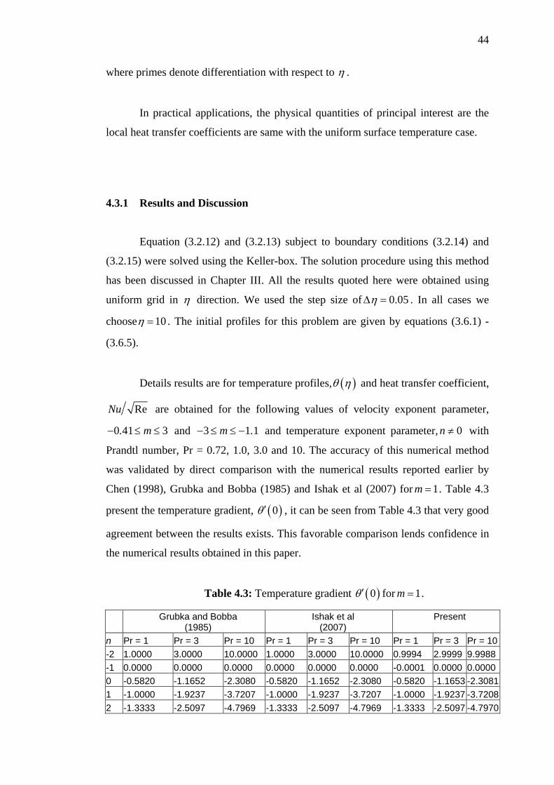
4.3 Temperature gradient ( )0θ ′ for 1m = . 44

4.4 Temperature gradient ( )0θ ′ as a function of Prandtl

numbers, temperature exponent and velocity exponent.

45

5.1 Comparison of heat transfer rate ( )' 0θ for λ = 0 and

various values of Pr.

59

5.2 Values of ( )'' 0f and ( )' 0θ for critical values of cλ (<0)

and different values of Pr.

60

5.3 Values of mean heat transfer rate ( )' 0Θ and the mean skin

friction rate ( )'' 0F for Pr = 0.72 and cλ = -0.13.

62

5.4 Values of mean heat transfer rate ( )' 0Θ and the mean skin

friction rate ( )'' 0F for Pr = 6.8 and cλ = -2.93.

63

viii

LIST OF FIGURES FIGURE NO. TITLE PAGE

3.1 Schematic diagram of flow induced by a continuous

stretching surface.

17

3.2 Net rectangle for difference approximations. 20

3.3 Flow diagrams for the Keller-box method. 36

3.4 Flow diagrams for the Keller-box method (continued). 37

4.1 Dimensionless temperature profiles, ( )θ η for various

values of Prandtl numbers for 3 and 0m n= = .

41


values of m for 0 and Pr 0.72n = = .

42

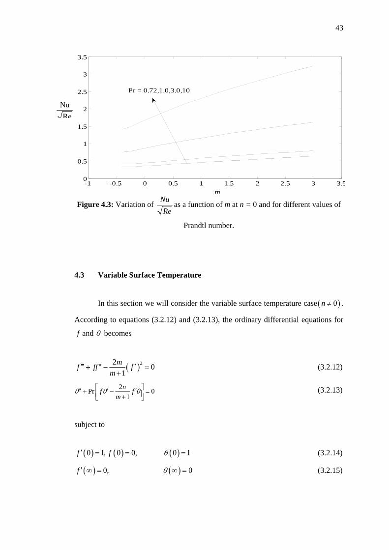
4.3 Variation of Nu

Reas a function of m at n = 0 and for

different values of Prandtl number.

43


values of n for 3 and Pr 0.72m = = .

48


values of Prandtl numbers for 0.25 and 1m n= − = − .

48

4.6 Variation of Nu

Reas a function of m at n = -1 and for


49

4.7 Variation of Nu

Reas a function of m at n = 2 and for


50


values of m for and Pr 0.72= .

53

ix


values of Prandtl number and 0.41m = − .

53

4.10 Variation of Nu

Reas a function of m at different values

of Prandtl number.

54

5.1 Physical model and coordinate system. 59

5.2 Variations of the skin friction with λ for different

values of Pr.

60

5.3 Variations of the heat flux with λ for different values of

Pr.

61

5.4 Variations of reduced skin friction rate for cλ = -0.13,

Pr = 0.7 and different values ofε .

64

5.5 Variations of heat flux on the wall for cλ = -0.13, Pr =

0.7 and different values ofε .

64

5.6 Variations of reduced skin friction withτ for 93.2−=cλ ,

Pr = 6.8 and different values ofε .

65

5.7 Variations of heat flux on the wall with for, Pr = 6.8

and different values ofε .

65

5.8 Variations of reduced skin friction with τ for ε = 0.5,

Pr = 0.72 and different values ofλ .

66

5.9 Variations of heat flux on the wall with τ for ε = 0.5,


66

5.10 Variations of reduced skin friction with τ for ε = 0.5,


67

5.11 Variations of heat flux on the wall with τ for ε = 0.5,


67

x

LIST OF SYMBOLS C - dimensional constant

d - dimensionless injection or suction parameter

f - dimensionless stream function

m - velocity exponent parameter

n - temperature exponent parameter

Nu - Nusselt number

Pr - Prandtl number

Re - Reynolds number

T - temperature

u - velocity component in x-direction

0U - dimensional constant

v - velocity component in y-direction

x - coordinate in direction of surface motion

y - coordinate in direction normal to surface motion

Greek symbols

α - thermal diffusivity

η - dimensionless similarity variable

θ - dimensionless temperature

ν - kinematic viscosity

ψ - stream function

Subscripts

w - condition at the surface

∞ - condition at ambient medium

Superscripts

‘ - differentiation with respect to η

CHAPTER I

INTRODUCTION 1.1 Heat Transfer on Continuous Stretching Surface

Heat transfer is the energy interaction due to a temperature difference in a

medium or between media. Heat is not a storable quantity and is defined as energy in

transit due to a temperature difference. The applications of heat transfer are diverse,

both in nature and in industry. Climatic changes, formation of rain and snow, heating

and cooling of the earth surface, the origin of dew drops and fog, spreading of forest

fires are some of the natural phenomena wherein heat transfer plays a dominant role.

The importance of heat transfer in industry include heating and air conditioning of

building, design of internal combustion engines, oil exploration, drying and

processing of solid and liquid wastes.

It is no wonder J.B Joseph Fourier, the father of the theory of heat diffusion,

made this remark in 1824: ‘Heat, like gravity, penetrates every substance of the

universe; its rays occupy all parts of space. The theory of heat will hereafter forms

one of the most important branches of general physics’, (Ghoshdastidar (2004)).

The problem of flow and heat transfer adjacent to a continuous stretching

surface has attracted many researchers during the past few decades. This is because

of its wide application in many manufacturing processes, such as continuous casting,

glass fiber production, metal extrusion, hot rolling, manufacturing of plastic, paper

production and wire drawing, (Chen (2000)). Both the kinematics of stretching and

the heat transfer during such process have a decisive influence on the quality of the

final product.

2

1.2 g-Jitter and Its Effects

Space experiments have revealed unknown or nonexistent effects on Earth

which can be detrimental to certain experiments. For example, alloy solidification

experiments conducted in space vehicles showed that the solute uniformity and

defects formation in space grown crystals are strongly affected by free convection in

the melt pool that arises as a result of the combined action of temperature and

concentration gradients in the melt (Nelson (1991), Monti and Sovino (1998),

Wilcox and Regel (2001)). These deleterious effects generally are considered to be a

culprit for the quality of crystals grown in low-gravity environments (Alexander et.

al. (1991), Kamotani et.al. (1995), Neumann (1990)). One of these effects is g-jitter

or residual acceleration phenomena associated with the microgravity environment.

g-Jitter is defined as the inertia effects due to quasi-steady, oscillatory or

transient accelerations arising from crew motions and machinery vibrations in

parabolic aircrafts, space shuttles or other microgravity environments. Quasi-steady

accelerations are accelerations which vary only little for periods longer than one

minute, oscillatory accelerations are periodic with a characteristic frequency, while

transient accelerations are non-periodic and typically have duration less than one

second (Mell (2001)). g-Jitter characterizes a small fluctuating gravitational field,

very irregular in amplitude, random in direction, and contains a broad spectrum of

frequencies (Schneider and Straub (1989), Alexander et.al. (1991), Nelson (1991)).

Its effects may be negligible in earthbound situations, but in a low-gravity

environment, where heat and mass transfer in a fluid medium, in the absence of

radiation, is expected to be affected only by pure diffusion, g-jitter can give rise to

significant convective motions.

Studies on g-jitter effects indicate that convection in microgravity is related to

the magnitude and frequency of g-jitter and to the alignment of the gravity field with

respect to the growth direction or the direction of the temperature gradient (Pan et. al.

(2002), Shu et. al (2001)). As an example, Ramos (2000) has shown that the

thickness and axial velocity components, heat fluxes and interfacial temperature are

3

periodic functions of time whose amplitudes increase as the amplitude of the g-jitter

increases, but decrease as the frequency of g-jitter increases. Results from Li (1996)

show that the frequency and amplitude of the g-jitter all play an important role in

determining the convective flow behaviour of the system. When the residual

accelerations oscillate about the positive and negative of an axis, the orientation of

this direction relative to the density gradient determines whether a mean flow is

generated in the system.

g-Jitter has large effects on materials processing in space or in gravity-

reduced environment. It can interact with the density gradients and result in both

fluid flow and solute segregation. Wilcox and Regel (2001) has reviewed the

microgravity effects on the material processing. They concluded that convection

should result, that the amount of convection increases with increasing acceleration

and decreasing frequency, and that it will significantly influence some materials

processing operations. Alexander et al. (1991) found that the orientation of the

residual gravity is a crucial factor in determining the suitability of the spacecraft

environment as a means to suppress or eliminate unwanted effects caused by buoyant

fluid motion in Bridgman's crystal growth experiment. These authors found that g-

jitter affects the compositional uniformity of the growing crystal.

1.3 Significance of Research

The effect of g-jitter on experiments, compared to ideal zero gravity

conditions, is largely unknown, especially in quantitative terms. It is therefore of

great interest to quantitatively access acceptable acceleration levels for a given

experiment such that the processes to be studied would not be appreciably distorted

by the environment in which the experiments take place. Significant levels of g-jitter

have been detected during space missions in which low-gravity experiments were

being conducted. The problem has been approached from a numerical standpoint,

one of the key results being that a relatively modest acceleration of 10-5g0 (g0 being

the gravity on the surface or the Earth) can have a significant impact on solute

4

segregation (Pan et. al (2002)). This is true even though velocity magnitudes are

several orders lower than under terrestrial conditions. Unfortunately, a complete

experimental parametric study of this g-jitter problem is obviously impossible, so

one has to rely on modelling to gain some insight into the question (Alexander et. al.

(1991)).

Alexander (1997) has mentioned that theoretical models can be used

effectively to predict the experiment sensitivity to g-jitter, provided the time-

dependent nature of the g-jitter is properly characterized. His experimental work in

the MEPHISTO (Material pour l'Etude des Phenomenes Interessant la Solidification

sur Terre et n Orbite) furnace facility to observe the effect of g-jitter on segregation

during directional solidification of tin-bismuth indicated that a "cause and effect"

relationship between g-jitter and disturbances in the transport conditions can be

clearly identified. These results are of significance for planning future low-gravity

experiments, and analyzing the results of past experiments. Reliable prediction of g-

jitter sensitivity based on models with proven experimental correlations can be used

to optimize the limited time available for low-gravity experimentation, determine

acceptable levels of g-jitter, and avoid unnecessary (expensive) design restrictions

which might arise due to inaccurate predictions.

For materials science experiments conducted in low earth-orbit spacecraft,

there are many open questions regarding experiment sensitivity to residual

acceleration. Since sensitivity to g-jitter is an important consideration in the selection

of optimal experiment operating conditions, it is imperative that these questions be

answered so that the scientific return from such experiments is maximized. In order

to obtain a more efficient engineering design in low-gravity conditions, more

informations regarding the effect of g-jitter on fluid behaviour in low gravity

environment is needed. The results of study should be helpful in understanding the g-

jitter effects on fluid mechanics process in microgravity conditions and better

engineering design could be made in the future.

5

1.4 Objectives and Scope of Research

The main objective of this project is to investigate theoretically the heat

transfer coefficients on continuous stretching surface and the effect of g-jitter

adjacent to a vertical stretching sheet. This involves the construction of suitable

mathematical models by formulating the appropriate governing equations and

choosing the right boundary conditions and then solving the resulting equations using

both analytical and numerical means.

1.5 Report Outline

This report consists of six chapters including this introductory chapter, where

we have presented the research background, objectives and significance of research.

In Chapter 2, a literature review on the problems concerning the heat transfer on

continuous stretching surface and the effect of g-jitter adjacent to a vertical

stretching sheet presented and discussed. Chapter 3, concerned with numerical

scheme used in this study, which is the Keller-box method. Keller and Cebeci

(1972) reported that this method is very simple and accurate which is applicable to

boundary layer flow problems. This method is chosen since it seem to be most

flexible of the common methods, being easily adaptable to solving equation of any

order (Cebeci and Bradshaw (1977)). One of the basic ideas of the Keller-box

method is to write the governing equation in the form of a first order system.

In Chapter 4, we consider the problem of heat transfer coefficients on a

continuous stretching surface. We will use the Keller-box method that has been

described in Chapter 3 to solve this problem. Three cases of thermal boundary

conditions, namely uniform surface temperature ( )0n = , variable surface

temperature ( )0n ≠ and uniform heat flux ( )( )1 2n m= − are presented in the

following three main section.

6

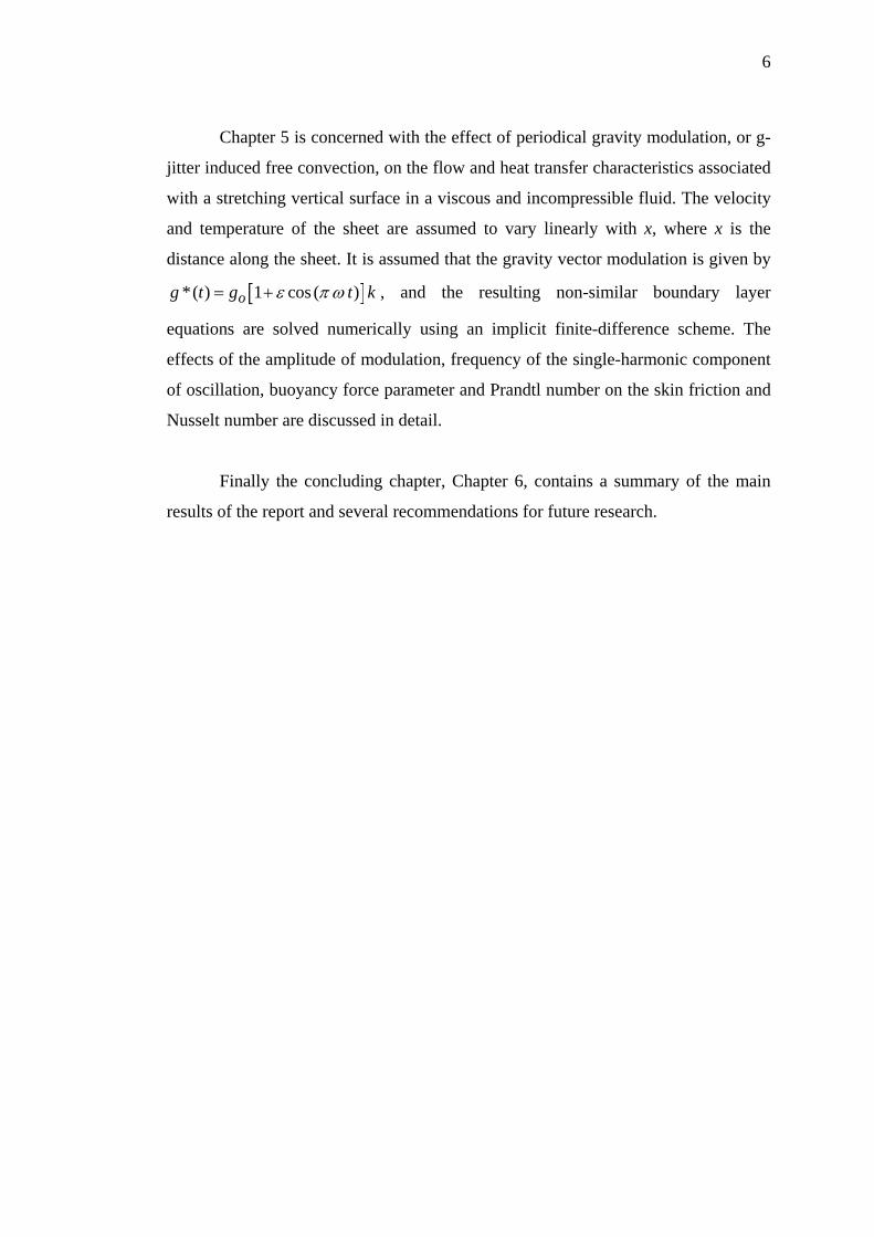
Chapter 5 is concerned with the effect of periodical gravity modulation, or g-

jitter induced free convection, on the flow and heat transfer characteristics associated

with a stretching vertical surface in a viscous and incompressible fluid. The velocity

and temperature of the sheet are assumed to vary linearly with x, where x is the

distance along the sheet. It is assumed that the gravity vector modulation is given by

[ ]*( ) 1 cos ( )og t g t kε π ω= + , and the resulting non-similar boundary layer

equations are solved numerically using an implicit finite-difference scheme. The

effects of the amplitude of modulation, frequency of the single-harmonic component

of oscillation, buoyancy force parameter and Prandtl number on the skin friction and

Nusselt number are discussed in detail.

Finally the concluding chapter, Chapter 6, contains a summary of the main

results of the report and several recommendations for future research.

CHAPTER II

LITERATURE REVIEW 2.1 Introduction This chapter contains a literature review on two main topics to be

investigated, namely in Section 2.2 studies concerning with continuous stretching

surface is discussed and in Section 2.3 contains related research on the effect of g-

jitter on vertical stretching sheet.

2.2 Continuous Stretching Surface

The flow and heat transfer stirred up by a continuous stretching surface

entering the cooling viscous fluid is important in a practical engineering process. For

example, materials which are manufactured by extrusion process and heat-treated

substances proceeding between a feed roll and a wind-up roll can be classified as the

continuous stretching surface. In order to get the top-grade property of the final

product, the cooling procedure should be effectively controlled. There are three types

of velocity and temperature distributions for problems involving continuous

stretching surface namely self similar, power law and exponential form.

In the past few decades, the related investigation about stretching surface has

never been interrupted. Sakiadis (1961) initiated the study of boundary layer flow

over a continuous solid surface moving with constant speed. It was observed that the

boundary layer growth is in the direction of motion of the continuous solid surface

8

and different from that of the Blasius flow past a flat plate. Crane (1970) gave

similarity solution closed to an analytical form for steady 2D incompressible

boundary layer flow caused by the stretching surface with linear velocity.

Banks (1983) discussed the flow field of stretching wall with a power law

velocity variation for different values of velocity exponent. Grubka and Bobba

(1985) studied the heat transfer characteristics of a continuous stretching surface

with linear surface velocity and power law surface temperature for different value of

Prandtl number and temperature exponent.

Ali (1994) who extended Bank’s and Grubka work for continuous stretching

surface problem. He investigates the heat transfer characteristics of a continuous

stretching surface with power law velocity and temperature distribution. Three

thermal boundary conditions of uniform surface temperature, variable surface

temperature and uniform heat flux at the continuous stretching surface had been

investigated.

Chen and Char (1988) has reported the heat transfer characteristics of a

continuous stretching surface with power law surface temperature and power law

surface heat flux variation with effect of suction or blowing. Ali (1995) has

examined the effects of suction or injection for heat and flow in a quiescent fluid

driven by a continuous stretched surface. He also used power law velocity and

temperature variation with three thermal boundary condition for this problem. The

thermal boundary condition that he used was the same with Ali (1994). It was shown

that suction increased the heat transfer from surfaces whereas, injection cause a

decrease in the heat transfer.

Rollins and Vajwavelu (1991) have investigated the heat transfer

characteristics in a viscoelastic fluid over a continuous stretching surface with

internal heat generation. Two cases were studied in this problem namely (i) the sheet

with uniform surface temperature and (ii) the sheet with uniform wall heat flux. The

solution and heat transfer characteristics were obtained in terms of Kummer’s

9

Functions. They found for large values of Prandtl number a uniform approximation

could be expressed in terms of parabolic cylinder functions in both cases.

Chen (1998) presented the numerical solutions of laminar mixed convection

in boundary layers adjacent to vertical, continuously stretching sheets. The Keller-

box method was used to solve this problem. The author studied the effect of thermal

buoyancy on flow past a vertical, continuously stretching where the velocity and

temperature variation was assumed power law form.

Magyari and Keller (1998) discussed heat and mass transfer in the boundary

layer on an exponentially stretching continuous surface. They intended to complete

the investigations by discussing a further type of similarity solution of the governing

equations. Their solutions involve an exponential dependence of the similarity

variable as well as the stretching velocity and the temperature distribution on the

coordinate in the direction parallel to that of the stretching.

In 2001, Mohammadein and Rama studied the heat transfer characteristics of

a laminar micropolar fluid boundary layer over a linearly stretching, continuous

surface. They consider the effect of viscous dissipation and internal heat generation

with self similar velocity and temperature variation.

Heat transfer characteristic of the separation boundary flow induced by a

continuous stretching surface was reported by Magyari and Keller (1999). They

discussed an exact-solvable case of separation flow characterized by an identically

vanishing skin friction with power law velocity and temperature variation.

Tashtoush et al (2000) have examined the laminar boundary layer flow and

heat transfer characteristics of a non-Newtonian fluid over a continuous stretching

surface subject to power-law velocity and temperature distribution with suction or

injection parameter. Their results was obtained numerically using fourth order

Rungge-Kutta method to show suction and injection effect for uniform and cooled

surface temperature.

10

Chen (2000) have investigated the flow and heat transfer characteristics

associated with a heated, continuously stretching surface being cooled by a mixed

convection flow. These problems also assume the velocity and temperature

distribution is varying according to a power-law form subject to variable surface

temperature and variable surface heat flux boundary condition. Their results show

that the local Nusselt number is increased with increasing the velocity exponent for

variable surface temperature case while the opposite trend is observed for the

variable surface heat flux. The author also found that the local skin friction

coefficient is increased for a decelerated stretching surface, while it decreased for an

accelerated stretching surface.

Mechanical and thermal properties of the self similar boundary layer flow

induced by continuous stretching surface with rapidly decreasing power law

( )1m < − and exponential velocity was studied by Maygari et al (2001).Ali (2004)

who extend Magyari et al (2001) work for continuous stretching surface with

different values of velocity exponent in the presence of the buoyancy force and the

surface was moving vertically subject to power-law velocity.

Seddek and Salem (2005) examined the effect of thermal buoyancy on flow

past a vertical continuous stretching surface with variable viscosity and variable

thermal diffusivity. Their results showed that variable viscosity, variable thermal

diffusivity, the velocity exponent parameter, the temperature had the significance

influences on the velocity and temperature profiles, shear stress and Nusselt number

in two cases air and water. The result was obtained numerically using the shooting

method.

Partha et al (2005) presented a similarity solution for a mixed convection

flow and heat transfer from an exponentially stretching surface subject to

exponential velocity and temperature distribution. The influence of buoyancy along

with viscous dissipation on the convective transport in the boundary layer region is

analyzed.

11

Magyari and Keller (2006) studied the heat transfer characteristics of the

laminar boundary layer flow induced by continuous stretching surface with

prescribed skin friction subject to power law velocity and temperature variation.

Sanjayanand and Khan (2006) analyzed the effect of various physical

parameters like viscoelastic parameter, Prandtl number, local Reynold number and

Eckert number on various momentum, heat and mass transfer of boundary layer with

second fluid characteristic over continuous stretching surface with exponential

velocity and temperature distribution.

Recently Ishak et al (2007) studied the mixed convection on the stagnation

point flow toward a vertical, continuously stretching sheet. They analyzed the effects

of governing parameters on the flow and heat transfer characteristics for fixed value

of Prandtl number. They found the dual solution exist in the neighborhood of the

separation region.

Many authors have studied this problem. However they limited to some

constraints on the surface velocity and temperature. Tsou et al (1967) have

considered the continuous moving surface with constant velocity and temperature.

Stretched surface with different velocity boundary condition and for various

temperature boundaries at the surface was studied by Crane (1970), Grubka and

Bobba (1985), Soundalgekar and Murty (1980) and Vleggar (1977).

Suction or injection of a stretched surface was introduced by Erickson et al

(1966) and Fox et al (1968) for uniform surface velocity and temperature. Gupta and

Gupta (1977) extended Erickson’s work, in which the surface was moved with a

linear speed for various values of parameters. Furthermore, linearly stretching

surface subject to suction or injection was studied by Chen and Char (1998) for

uniform wall temperature and heat flux.

In the classical convective heat transfer between solid wall and the fluid flow,

usually the temperature or heat flux at the solid-fluid interface is prescribed over the

entire interface. Physically, the condition of uniform surface temperature is achieved

12

by either violent mixing or a phase change, for example, boiling or condensation, on

the other side of a thin wall that has a higher thermal conductivity. However, in

certain engineering systems, the condition of constant surface temperature does not

apply. For example, in the design of thermal insulation, material processing, and

geothermal systems, it has been observed that natural convection can induce thermal

stresses that lead to critical structural damage in the piping systems of nuclear

reactors. But, an important practical and experimental circumstance in many forced,

free and mixed convection flows is that generated adjacent to a surface dissipating

heat uniformly.

The effect of uniform surface temperature and uniform heat flux gives much

impact on heat transfer process. Thus, our first problem of this study is to investigate

the heat transfer coefficients of a continuous stretching surface subjected to a

uniform surface temperature, variable surface temperature and uniform heat flux,

respectively.

2.3 The Effect of g-Jitter on Vertical Stretching Sheet The production of sheeting material which includes both metal and polymer

sheets arises in a number of industrial manufacturing processes. The fluid dynamics

due to a stretching surface is important in many extrusion processes. Since the

pioneering study by Crane (1970) who presented an exact analytical solution for the

steady two-dimensional stretching of a surface in a quiescent fluid many authors

have considered various aspects of this problem and obtained similarity solutions.

Many researchers presented theoretical results on this problem. The papers by

Magyari and Keller (1999, 2000), and Nazar et al. (2004) contain a good amount of

references, but these studies pertain to forced convection flows only. On the other

hand, problems involving the boundary layer flow due to a stretching surface in the

vertical direction in a steady, viscous and incompressible fluid when the buoyancy

forces are taken into account have been considered by Daskalakis (1993), Ali and Al-

Yousef (1998), Chen (1998, 2000), Lin and Chen (1998) and Chamkha (1999).

13

However, only Kumari et al. (1996) have studied the unsteady free convection flow

over a stretching vertical surface in an ambient fluid, where they considered both

cases of constant surface temperature and constant heat flux.

It is known that in many situations the presence of a temperature gradient and

a gravitational field can generate buoyancy convective flows. Recent technological

implications have given rise to increased interest in oscillating natural and mixed

convection driven by g-jitter forces associated with microgravity. In low-gravity or

microgravity environments, it can be expected that the reduction or elimination of

natural convection may enhance the properties and performance of materials such as

crystals. However, aboard orbiting spacecrafts all objects experience low-amplitude

perturbed accelerations, or g-jitter, caused by crew activities, orbiter manoeuvres,

equipment vibrations, solar drag and other sources (Antar and Nuotio-Antar, (1993);

Hirata et al. (2001)). There is a growing literature, which tries to characterize the g-

jitter environment and the review articles by Alexander (1990) and Nelson (1991)

give a good summary of earlier work on convective flows in viscous fluids. There

have also been a number of studies which investigate the effect of g-jitter on flows

involving viscous fluids and porous media, e.g. Amin (1988), Farooq and Homsy

(1994), Li (1996), Pan and Li (1998), Rees and Pop (2000, 2001), and Chamkha

(2003). However, to our best knowledge there has not been any study regarding g-

jitter effects on stretching problems. Therefore, in this paper, we will study the

behavior of g-jitter induced free convection of a viscous and incompressible fluid

due to a surface, which is stretched in the vertical direction.

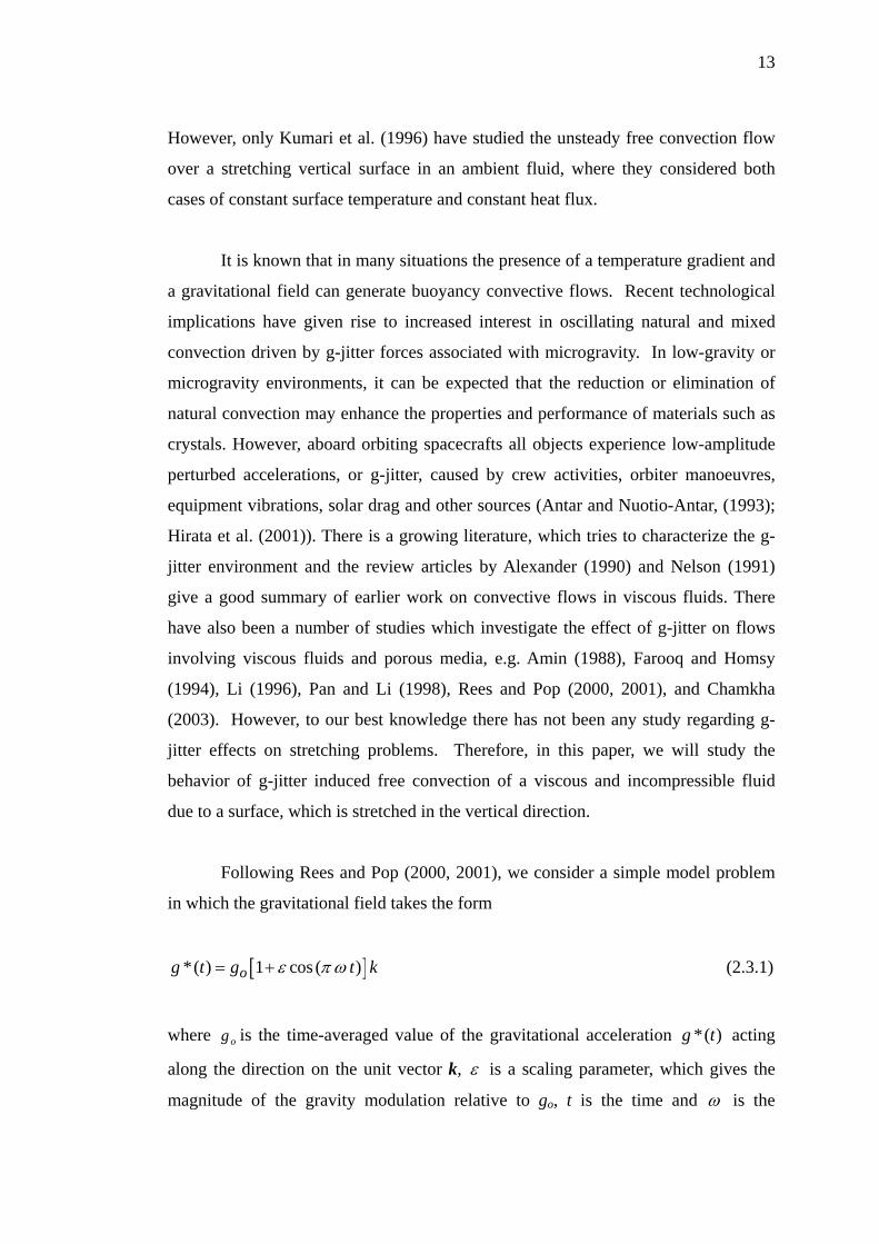
Following Rees and Pop (2000, 2001), we consider a simple model problem

in which the gravitational field takes the form

[ ]*( ) 1 cos ( )og t g t kε π ω= + (2.3.1)

where og is the time-averaged value of the gravitational acceleration *( )g t acting

along the direction on the unit vector k, ε is a scaling parameter, which gives the

magnitude of the gravity modulation relative to go, t is the time and ω is the

14

frequency of oscillation of the g-jitter driven flow.

The effect of oscillating free convection is driven by g-jitter forces associated

with a gravitational field given by equation (2.3.1) on the boundary layer flow over a

vertical stretching surface. For many practical applications the stretching surfaces

undergo cooling or heating that cause surface velocity and temperature variations. It

is assumed here that the stretching velocity and the surface temperature vary linearly

with the distance along the surface. In addition, it is assumed that the g-jitter field

under consideration is spatially constant , otherwise varies harmonically with time.

The governing partial differential equations are transformed into a non-dimensional

form using similarity variables and then solved numerically using the Keller-box

method which is an implicit finite-difference scheme.

Similarity solutions can be obtained for the special case when the amplitude

of the modulation is zero and we have shown that solutions of these equations exist

only for limited values of the negative buoyancy force parameter. Effects of the

amplitude of modulation, frequency of the single-harmonic component of oscillation,

buoyancy force parameter and Prandtl number on the skin friction and Nusselt

number are discussed in detail.

CHAPTER III

THE KELLER-BOX METHOD 3.1 Introduction This chapter discusses the details of the numerical scheme used in this study,

which is the Keller-box method. Keller and Cebeci (1972) reported that this method

is very simple and accurate which is applicable to boundary layer flow problems.

This method is chosen since it seem to be most flexible of the common methods,

being easily adaptable to solving equation of any order (Cebeci and Bradshaw

(1977)). One of the basic ideas of the Keller-box method is to write the governing

equation in the form of a first order system.

In Section 3.2 the discussion begins with the governing equations for the

problem of the heat transfer characteristic of a continuous stretching surface. Then

we discuss the finite difference method in Section 3.3. We shall use centered

difference derivatives and average at the midpoints of net rectangle to get the finite

difference equations. The finite difference equations are generally nonlinear

algebraic equations. In this study, we linearize the resulting nonlinear algebraic

equations using Newton’s method. Full details of Newton’s method will give in

Section 3.4. In Section 3.5, we solve the linear system by the block-tridiagonal

factorization method. This method is employed on the coefficient matrix of the finite

difference equations. Finally, we discuss the choice of suitable starting conditions

for the numerical computation in Section 3.6. This section include the determination

of values y∞ , the selection of step size, as well as the assumptions of the initial

velocity and temperature profiles.

16

3.2 Governing Equation A steady two dimensional motion of incompressible viscous fluid due to a

continuous stretching surface in a stationary fluid is governed by the continuity,

momentum and energy equation under the boundary layer approximation are

Continuity equation,

0u vx y∂ ∂

+ =∂ ∂

(3.2.1)

Momentum equation,

2

2

u u uu vx y y

ν∂ ∂ ∂+ =

∂ ∂ ∂ (3.2.2)

Energy equation,

2

2

T T Tu vx y y

α∂ ∂ ∂+ =

∂ ∂ ∂ (3.2.3)

subject to boundary conditions

( )wu u x= , 0v = and ( )wT T x= at 0,y = (3.2.4a)

0u = and T T∞= at y →∞ (3.2.4b)

The continuous stretching surface is assumed to have power-law velocity and

temperature variations, that is ( ) 0m

wu x U x= and ( ) nwT x T Cx∞= + where 0U and C

are constant and m and n are the velocity and temperature exponent parameter.

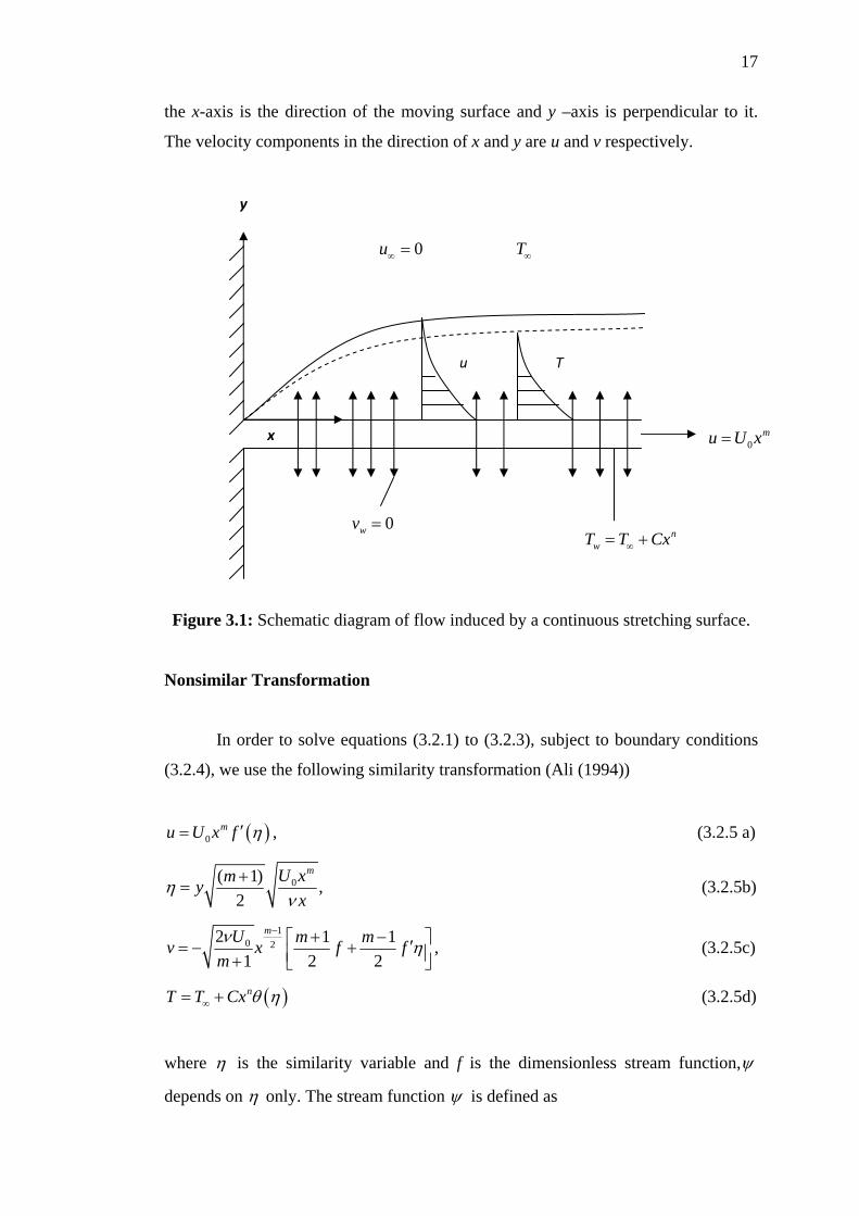
The Cartesian coordinates ( ),x y and the boundary layer representation on a

continuous stretching surface are shown schematically in Figure 3.1. In this figure

17

the x-axis is the direction of the moving surface and y –axis is perpendicular to it.

The velocity components in the direction of x and y are u and v respectively.

Figure 3.1: Schematic diagram of flow induced by a continuous stretching surface.

Nonsimilar Transformation

In order to solve equations (3.2.1) to (3.2.3), subject to boundary conditions

(3.2.4), we use the following similarity transformation (Ali (1994))

( )0mu U x f η′= , (3.2.5 a)

0( 1) ,2

mU xmyx

ην

+= (3.2.5b)

10 22 1 11 2 2

mU m mv x f fmν η

− + −⎡ ⎤′= − +⎢ ⎥+ ⎣ ⎦, (3.2.5c)

( )nT T Cx θ η∞= + (3.2.5d)

where η is the similarity variable and f is the dimensionless stream function,ψ

depends on η only. The stream function ψ is defined as

x

u T

0mu U x=

y

nwT T Cx∞= +

0wv =

0u∞ = T∞

18

,u vy xψ ψ∂ ∂

= = −∂ ∂

(3.2.6)

In terms of the stream function ψ , equations (3.2.2) and (3.2.3) become

2 2 3

2 3y x y x y yψ ψ ψ ψ ψν∂ ∂ ∂ ∂ ∂

− =∂ ∂ ∂ ∂ ∂ ∂

(3.2.7)

2

2

T T Ty x x y yψ ψ α∂ ∂ ∂ ∂ ∂

− =∂ ∂ ∂ ∂ ∂

(3.2.8)

From equations (3.2.5a, b), we obtain the chain rule following system of equations:

20

02

( 1)2

mm U xmU x f

y xψ

ν∂ +′′=∂

(3.2.9a)

30

03

1( )( )2

mm U xmU x f

y xψ

ν∂ +′′′=∂

(3.2.9b)

121 0 2

0 0( 1) ( 1)

2 2

mm m Um mU mx f U x y x f

x y xψ

ν

−−∂ + − ′= +

∂ ∂ (3.2.9c)

From equations (3.2.5c), ( )nT T Cx θ η∞= + , then

( )nT Cx θ ηθ∂

=∂

(3.2.10)

11 0 2( 1) ( 1)

2 2

mn n UT m mnCx Cx y x

xθ θ

ν

−−∂ + − ′= +

∂ (3.2.11a)

0( 1)2

mn U xT mCx

y xθ

ν∂ + ′=∂

(3.2.11b)

20

2

1( )( )2

mn U xT mCx

y xθ

ν∂ + ′′=∂

(3.2.11c)

Substituting equations (3.2.9) and (3.2.11) into equations (3.2.7) and (3.2.8), we

obtain the following system of equations:

19

( )22 01

mf ff fm

′′′ ′′ ′+ − =+

, (3.2.12)

2Pr 01

nf fm

θ θ θ⎡ ⎤′′ ′ ′+ − =⎢ ⎥+⎣ ⎦. (3.2.13)

subject to

( ) ( ) ( )0 1, 0 0, 0 1f f θ′ = = = , (3.2.14)

( ) ( )0, 0f θ′ ∞ = ∞ = . (3.2.15)

3.3 The Finite Difference Method To solve (3.2.12) and (3.2.13) using Keller-box method, we write equations

(3.2.12) and (3.2.13) as a system of first-order equations. For this purpose, we

introduce new dependent variable ( , ), ( , )u x y v x y and ( , )t x y and G replaces θ as the

variable for temperature. Therefore, we obtain

f u′ = u v′ = G t′ = (3.3.1a,b,c)

22 01

mv fv um

′ + − =+

(3.3.1d)

2Pr 01

nt ft uGm

⎡ ⎤′ + − =⎢ ⎥+⎣ ⎦ (3.3.1e)

where the primes denote differentiation with respect to η . In terms of the new

dependent variables, the boundary conditions become

( ),0 0, ( ,0) 1,f x u x= = ( ),0 1G x = (3.3.2a)

( ), 0u x ∞ = , ( ), 0v x ∞ = , ( , ) 0G x ∞ = (3.3.2b)

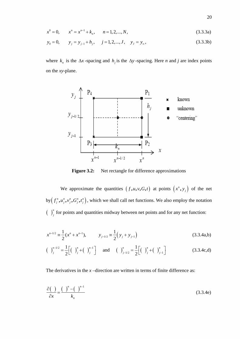
The net rectangle considered in the xy-plane is shown in Figure 3.1, and the

net points are denoted by:

20

0 10, , 1, 2,..., ,n nnx x x k n N−= = + = (3.3.3a)

0 10, , 1, 2,..., , ,j j j Jy y y h j J y y− ∞= = + = = (3.3.3b)

where nk is the xΔ -spacing and jh is the yΔ -spacing. Here n and j are index points

on the xy-plane.

Figure 3.2: Net rectangle for difference approximations

We approximate the quantities ( ), , , ,f u v G t at points ( ),njx y of the net

by ( ), , , ,n n n n nj j j j jf u v G t , which we shall call net functions. We also employ the notation

( )n

j for points and quantities midway between net points and for any net function:

( )1/2 11/2 1

1 1( ), 2 2

n n nj j jx x x y y y− −− −≡ + ≡ + (3.3.4a,b)

( ) ( ) ( ) ( ) ( ) ( )1/2 1

1/2 1

1 1 and 2 2

n n n n n n

j j j j j j

− −

− −⎡ ⎤ ⎡ ⎤= + = +⎣ ⎦ ⎣ ⎦ (3.3.4c,d)

The derivatives in the x –direction are written in terms of finite difference as:

( ) ( ) ( ) 1n n

nx k

−∂ −=

∂ (3.3.4e)

21

We write the difference equations that are to approximate equations (3.3.1a)

to (3.3.1e) by considering one mesh rectangle as in Figure 3.1. We start by writing

the finite difference approximations of the ordinary differential equations (3.3.1a) to

(3.3.1c) for the midpoint ( )1 2/,njx y − of the segment 1 2P P , using centered difference

derivatives. This process is called “centering about ( )1 2/,njx y − ”. We get

( ) ( )11 1/2

1 ,2

n nj j n n n

j j jj

f fu u u

h−

− −

−= + = (3.3.5a)

( ) ( )11 1/2

1 ,2

n nj j n n n

j j jj

u uv v v

h−

− −

−= + = (3.3.5b)

( ) ( )11 1/2

1 ,2

n nj j n n n

j j jj

G Gt t t

h−

− −

−= + = (3.3.5c)

Equations (3.3.1d,e) are approximated by centering the midpoint

( )1 21 2

//,n

jx y−− of the rectangle 1 2 3 4P P P P . This can be done in two steps. In the first

step, we center equations (3.3.1d,e) about the point ( )1 2/ ,nx y− without specifying y.

We denote the left-hand side of equations (3.3.1d,e) by 1 2 and L L , then the

approximations are

( )11 1

1 0,2

n nL L −+ = (3.3.6a)

( )12 2

1 0,2

n nL L −+ = (3.3.6b)

Rearranging equation (3.3.6) and using equation (3.3.4c), the difference

approximation to equations (3.3.1d,e) at 1 2/nx − become

( ) ( ) ( ) [ ] 121

2 ,1

nn n nmv fv u Lm

−′ + − = −+

(3.3.7a)

( ) ( ) ( ) [ ] 12

2Pr ,1

n n n nnt ft uG Lm

−⎡ ⎤′ + − = −⎢ ⎥+⎣ ⎦ (3.3.7b)

22

where

1 21

2 ,1

n mL v fv um

− ⎡ ⎤′= + −⎢ ⎥+⎣ ⎦ (3.3.8a)

12

2Pr ,1

n nL t ft uGm

− ⎡ ⎤⎡ ⎤′= + −⎢ ⎥⎢ ⎥+⎣ ⎦⎣ ⎦ (3.3.8b)

where the identity sign introduces useful shorthand: [ ] 1n− means that the quantities

in square bracket are evaluated at 1nx x −= .

The second step we center equations (3.3.7) about point ( )1/21/2,n

jx y−− by

using equation (3.3.4d) and we get

( ) ( ) [ ]2 111/2 1/2 1/2 1 1/2

2 ,1

n nnj j n n n

j j j jj

v v mf v u Lh m

−−− − − −

−+ − = −

+ (3.3.9a)

( ) [ ] 111/2 1/2 1/2 1/2 2 1/2

2Pr ,1

n nnj j n n n n

j j j j jj

t t nf t u G Lh m

−−− − − − −

− ⎡ ⎤+ − = −⎢ ⎥+⎣ ⎦ (3.3.9b)

where

[ ] ( ) ( )1

21 11 1/2 1/2 1/21/2

,

n

n j jj j jj

j

v vL f v u

h

−

− −− − −−

⎡ ⎤−⎢ ⎥= + −⎢ ⎥⎣ ⎦

[ ] ( ) 11 12 1/2 1/2 1/2 1/21/2

Pr ,nn j j

j j j jjj

t tL f t u G

h−− −

− − − −−

−⎡ ⎤= + −⎣ ⎦

Equations (3.3.5) and (3.3.9) are imposed for 1 2, , ...,j J= at given n, and the

transformed boundary layer thickness, Jy , is to be sufficiently large so that it is

beyond to the edge of the boundary layer by Keller and Cebeci (1972).

At nx x= , the boundary conditions (3.3.2) become

23

0 0 00, 1, 1, 0, 0, 0n n n n n nj j jf u G u v G= = = = = = (3.3.10)

3.4 Newton’s Method If we assume 1 1 1 1 1, , , ,n n n n n

j j j j jf u v G t− − − − − to be known for 0 j J≤ ≤ , then

equations (3.3.5), (3.3.9) and (3.3.10) are a system of equations for the solution of

the unknowns ( ), , , ,n n n n nj j j j jf u v G t , 0 1, , ...,j J= . For simplicity of notation we shall

write the unknowns at nx x= as

( ) ( ), , , , , , , ,n n n n nj j j j j j j j j jf u v G t f u v G t=

Then the system of equations (3.3.5) and (3.3.9) can be written as

( )1 1 0,2

jj j j j

hf f u u− −− − + = (3.4.1a)

( )1 1 0,2

jj j j j

hu u v v− −− − + = (3.4.1b)

( )1 1 0,2

jj j j j

hG G t t− −− − + = (3.4.1c)

( ) ( )( ) ( ) ( )2 11 1 1 1 1 1/2

2 ,4 1 4

nj jj j j j j j j j j

h hmv v f f v v u u Rm

−− − − − −

⎛ ⎞− + + + − + =⎜ ⎟+ ⎝ ⎠

(3.41d)

( ) ( )( )

( )( ) ( )

1 1 1

11 1 2 1/2

Pr4

2Pr1 4

jj j j j j j

njj j j j j

ht t f f t t

hn u u G G Rm

− − −

−− − −

⎡ ⎤− + + +⎢ ⎥

⎣ ⎦⎡ ⎤⎛ ⎞

− + + =⎢ ⎥⎜ ⎟+ ⎝ ⎠⎣ ⎦

(3.4.1e)

where

( ) ( ) ( )1

21 11 1/2 1/2 1/21/2

2 ,1

n

n j jj j j jj

j

v v mR h f v uh m

−

− −− − −−

⎡ ⎤−⎢ ⎥= + −

+⎢ ⎥⎣ ⎦ (3.4.2a)

24

( ) ( ) 1

1 12 1/2 1/2 1/2 1/21/2

2Pr ,1

n

n j jj j j j jj

j

t t nR h f t u Gh m

−

− −− − − −−

⎡ ⎤− ⎡ ⎤⎢ ⎥= − + −⎢ ⎥+⎣ ⎦⎢ ⎥⎣ ⎦ (3.4.2b)

( ) ( )1 11 21/2 1/2

and n n

j jR R− −

− − involves only known quantities if we assume that the solution

is known on 1nx x −= . To solve equation (3.4.1) with (3.3.10) by Newton’s method,

we introduce the iterates ( ) ( ) ( ) ( ) ( ), , , , , 0,1,2,...i i i i ij j j j jf u v G t i⎡ ⎤ =⎣ ⎦ .

In order to linearize the nonlinear system of equations (3.4.1) using Newton’s

method, we introduce the following iterates

( ) ( ) ( ) ( ) ( ) ( ) ( ) ( ) ( )

( ) ( ) ( ) ( ) ( ) ( )

1 1 1

1 1

, ,

, .

i i i i i i i i ij j j j j j j j j

i i i i i ij j j j j j

f f f u u u v v v

G G G t t t

δ δ δ

δ δ

+ + +

+ +

= + = + = +

= + = + (3.4.3)

Then we substitute (3.4.3) into (3.4.1) except the term on 1nx − , we get

( ) ( )( ) ( ) ( )( ) ( ) ( ) ( ) ( )( )1 1 1 1 0,2

ji i i i i i i ij j j j j j j j

hf f f f u u u uδ δ δ δ− − − −+ − + − + + + =

( ) ( )( ) ( ) ( )( ) ( ) ( ) ( ) ( )( )1 1 1 1 0,2


hu u u u v v v vδ δ δ δ− − − −+ − + − + + + =

( ) ( )( ) ( ) ( )( ) ( ) ( ) ( ) ( )( )1 1 1 1 0,2


hG G G G t t t tδ δ δ δ− − − −+ − + − + + + =

( ) ( )( ) ( ) ( )( ) ( ) ( ) ( ) ( )( ) ( ) ( ) ( ) ( )( )( ) ( ) ( ) ( )( ) ( )

1 1 1 1 1 1

2 11 1 1 1/2

42 ,

1 4

ji i i i i i i i i i i ij j j j j j j j j j j j

nj i i i ij j j j j

hv v v v f f f f v v v v

hm u u u u Rm

δ δ δ δ δ δ

δ δ

− − − − − −

−− − −

+ − + + + + + + + +

⎛ ⎞− + + + =⎜ ⎟+ ⎝ ⎠

( ) ( )( ) ( ) ( )( ) ( ) ( ) ( ) ( )( ) ( ) ( ) ( ) ( )( )( ) ( ) ( ) ( )( ) ( ) ( ) ( ) ( )( ) ( )

1 1 1 1 1 1

11 1 1 1 2 1/2

Pr4

2Pr ,1 4

ji i i i i i i i i i i ij j j j j j j j j j j j

nj i i i i i i i ij j j j j j j j j

ht t t t f f f f t t t t

hn u u u u G G G G Rm

δ δ δ δ δ δ

δ δ δ δ

− − − − − −

−− − − − −

⎡ ⎤+ − + + + + + + + +⎢ ⎥

⎣ ⎦⎡ ⎤⎛ ⎞

− + + + + + + =⎢ ⎥⎜ ⎟+ ⎝ ⎠⎣ ⎦

25

Next we drop the terms that are quadratic in ( ) ( ) ( ) ( ) ( )( ), , , ,i i i i ij j j j jf u v G tδ δ δ δ δ

and we have also drop the superscript I for simplicity. After some algebraic

manipulations, the following linear tridiagonal system of equations is obtained

( ) ( )1 1 1 1/2

1 ,2j j j j j j

f f h u u rδ δ δ δ− − −− − + = (3.4.4a)

( ) ( )1 1 2 1/2

1 ,2j j j j j j

u u h v v rδ δ δ δ− − −− − + = (3.4.4b)

( ) ( )1 1 3 1/2

1 ,2j j j j j j

G G h t t rδ δ δ δ− − −− − + = (3.4.4c)

( ) ( ) ( ) ( ) ( )( ) ( )1 2 1 3 4 1 5

6 1 4 1/2,

j j j j jj j j j j

jj j

a v a v a f a f a u

a u r

δ δ δ δ δ

δ

− −

− −

+ + + +

+ = (3.4.4d)

( ) ( ) ( ) ( ) ( )( ) ( ) ( ) ( )1 2 1 3 4 1 5

6 1 7 8 1 5 1/2,

j j j j jj j j j j

j j jj j j j

b t b t b f b f b u

b u b G b G r

δ δ δ δ δ

δ δ δ

− −

− − −

+ + + +

+ + + = (3.4.4e)

where

( )1 1/21 ,2

jjj

ha f −= +

( ) ( )2 1/2 11 2,2

jjj j

ha f a−= − + = − (3.4.5)

( ) ( ) ( )3 1/2 4 3, ,2

jjj j j

ha v a a−= =

( ) ( ) ( )5 1/2 6 52 , ,

1 j jj j j

ma h u a am −= − =+

( )1 1/2Pr1 ,2 j jj

b h f −= +

( ) ( )2 1/2 1Pr1 2,2 j jj j

b h f b−= − + = −

( ) ( ) ( )3 1/2 4 3Pr , ,2 j jj j j

b h t b b−= = (3.4.6)

( ) ( ) ( )5 1/2 6 5Pr , ,1 j jj j j

nb h G b bm −

⎛ ⎞= − =⎜ ⎟+⎝ ⎠

26

( ) ( ) ( )7 1/2 8 7Pr , ,1 j jj j j

nb h u b bm −

⎛ ⎞= − =⎜ ⎟+⎝ ⎠

( )1 1 1/21/2,j j j jj

r f f h u− −−= − +

( )2 1 1/21/2,j j j jj

r u u h v− −−= − +

( )3 1 1/21/2,j j j jj

r G G h t− −−= − + (3.4.7)

( ) ( ) 24 1 1/2 1/2 1/2

2 ,1j j j j j jj

mr v v h f v um− − − −

⎛ ⎞= − − − +⎜ ⎟+⎝ ⎠

( ) ( )5 1 1/2 1/2 1/2 1/22Pr ,

1j j j j j j jj

nr t t h f t u Gm− − − − −

⎛ ⎞= − − − +⎜ ⎟+⎝ ⎠

To complete the system (3.4.4), we recall the boundary condition (3.3.10),

which can be satisfied exactly with no iteration. So, to maintain these correct values

in all the iterates, we take

0 0 00, 0, 0, 0, 0, 0J J Jf u G u v Gδ δ δ δ δ δ= = = = = = (3.4.8)

3.5 Block-elimination Method The linear system (3.4.4) can be solved by the block-elimination method. The

linearized difference equations of the system (3.4.4) have a block-tridiagonal

structure.

Generally, the block-tridiagonal structure consists of variable or constant, but

here, an interesting feature can be observed that is, for the Keller-box method it

consists of block matrices. Before we solved the linear system (3.4.4) using block-

elimination method, we will show how to get the elements of the block matrices from

the linear system (3.4.4). We consider three cases, namely when 1 1 and ,j J J= − .

When 1j = , the linear system (3.4.4) become

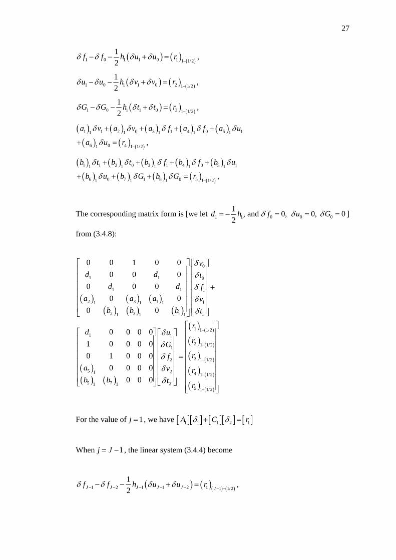
27

( ) ( ) ( )1 0 1 1 0 1 1 1/2

1 ,2

f f h u u rδ δ δ δ−

− − + =

( ) ( ) ( )1 0 1 1 0 2 1 1/2

1 ,2

u u h v v rδ δ δ δ−

− − + =

( ) ( ) ( )1 0 1 1 0 3 1 1/2

1 ,2

G G h t t rδ δ δ δ−

− − + =

( ) ( ) ( ) ( ) ( )( ) ( ) ( )

1 1 2 0 3 1 4 0 5 11 1 1 1 1

6 0 41 1 1/2,

a v a v a f a f a u

a u r

δ δ δ δ δ

δ−

+ + + +

+ =

( ) ( ) ( ) ( ) ( )( ) ( ) ( ) ( ) ( )

1 1 2 0 3 1 4 0 5 11 1 1 1 1

6 0 7 1 8 0 51 1 1 1 1/2,

b t b t b f b f b u

b u b G b G r

δ δ δ δ δ

δ δ δ−

+ + + +

+ + + =

The corresponding matrix form is [we let 1 11 ,2

d h= − 0and 0,fδ = 0 00, 0u Gδ δ= = ]

from (3.4.8):

( ) ( ) ( )( ) ( ) ( )

( )( ) ( )

( ) ( )

( ) ( )

( ) ( )

( ) ( )

( )

0

1 1 0

1 1 1

2 3 1 11 1 1

2 3 1 11 1 1

1 1 1/21 1

2 1 1/21

32 1 1/2

5 21 4 1 1/2

5 7 21 15 1

0 0 1 0 00 0 0

0 0 00 0

0 0

0 0 0 01 0 0 0 00 1 0 0 0

0 0 0 00 0 0

vd d t

d d fa a a v

b b b t

rd u

rGrf

a v rb b t r

δδδδδ

δδδδδ

−

−

−

−

⎡ ⎤ ⎡ ⎤⎢ ⎥ ⎢ ⎥⎢ ⎥ ⎢ ⎥⎢ ⎥ ⎢ ⎥ +⎢ ⎥ ⎢ ⎥⎢ ⎥ ⎢ ⎥⎢ ⎥ ⎢ ⎥⎣ ⎦⎣ ⎦

⎡ ⎤ ⎡ ⎤⎢ ⎥ ⎢ ⎥⎢ ⎥ ⎢ ⎥⎢ ⎥ ⎢ ⎥ =⎢ ⎥ ⎢ ⎥⎢ ⎥ ⎢ ⎥⎢ ⎥ ⎢ ⎥⎣ ⎦⎣ ⎦

( )1/2−

⎡ ⎤⎢ ⎥⎢ ⎥⎢ ⎥⎢ ⎥⎢ ⎥⎢ ⎥⎢ ⎥⎢ ⎥⎣ ⎦

For the value of 1j = , we have [ ][ ] [ ][ ] [ ]1 1 1 2 1A C rδ δ+ =

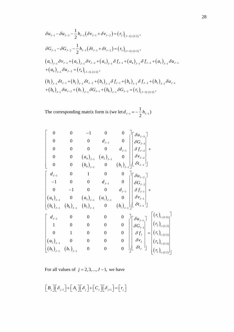
When 1j J= − , the linear system (3.4.4) become

( ) ( )( ) ( )1 2 1 1 2 1 1 1/2

1 ,2J J J J J J

f f h u u rδ δ δ δ− − − − − − −− − + =

28

( ) ( )( ) ( )1 2 1 1 2 2 1 1/2

1 ,2J J J J J J

u u h v v rδ δ δ δ− − − − − − −− − + =

( ) ( )( ) ( )1 2 1 1 2 3 1 1/2

1 ,2J J J J J J

G G h t t rδ δ δ δ− − − − − − −− − + =

( ) ( ) ( ) ( ) ( )( ) ( )( ) ( )

1 1 2 2 3 1 4 2 5 11 1 1 1 1

6 2 41 1 1/2,

J J J J JJ J J J J

JJ J

a v a v a f a f a u

a u r

δ δ δ δ δ

δ− − − − −− − − − −

−− − −

+ + + +

+ =

( ) ( ) ( ) ( ) ( )( ) ( ) ( ) ( )( ) ( )

1 1 2 2 3 1 4 2 5 11 1 1 1 1

6 2 7 1 8 2 51 1 1 1 1/2,

J J J J JJ J J J J

J J JJ J J J

b t b t b f b f b u

b u b G b G r

δ δ δ δ δ

δ δ δ− − − − −− − − − −

− − −− − − − −

+ + + +

+ + + =

The corresponding matrix form is (we let 1 112J Jd h− −= − )

( ) ( )( ) ( )

( ) ( ) ( )( ) ( ) ( ) ( )

3

1 3

1 2

24 21 1

24 21 1

1 2

1 2

1

6 3 11 1 1

6 8 3 11 1 1 1

0 0 1 0 0

0 0 0 0

0 0 0 0

0 0 0

0 0 0

0 1 0 0

1 0 0 0

0 1 0 0

0 0

0

J

J J

J J

JJ J

JJ J

J J

J J

J

J J J

J J J J

ud G

d fva atb b

d ud G

d

a a a

b b b b

δδδδδ

δδ

−

− −

− −

−− −

−− −

−−

− −

−

− − −

− − − −

⎡ ⎤− ⎡ ⎤⎢ ⎥ ⎢ ⎥⎢ ⎥ ⎢ ⎥⎢ ⎥ ⎢ ⎥ +⎢ ⎥ ⎢ ⎥⎢ ⎥ ⎢ ⎥⎢ ⎥ ⎢ ⎥⎣ ⎦⎢ ⎥⎣ ⎦⎡ ⎤⎢ ⎥

−⎢ ⎥⎢ ⎥−⎢ ⎥⎢ ⎥⎢ ⎥⎢ ⎥⎣ ⎦

( )( ) ( )

( ) ( )

( ) ( )

( ) ( )

( ) ( )

( ) ( )

1

1

1

1 1 1/21 1

2 1 1/21

3 1 1/2

5 41 1 1/2

5 71 1 5 1 1/2

0 0 0 0

1 0 0 0 0

0 1 0 0 0

0 0 0 0

0 0 0

J

J

J

J J

J

J

JJ

JJ J

fvt

rd urGrf

va rtb b r

δδδ

δδδδδ

−

−

−

−−−

−−

−

− −

− − −

⎡ ⎤⎢ ⎥⎢ ⎥⎢ ⎥ +⎢ ⎥⎢ ⎥⎢ ⎥⎣ ⎦

⎡ ⎤⎡ ⎤ ⎡ ⎤ ⎢ ⎥⎢ ⎥ ⎢ ⎥ ⎢ ⎥⎢ ⎥ ⎢ ⎥ ⎢ ⎥⎢ ⎥ ⎢ ⎥ ⎢ ⎥=⎢ ⎥ ⎢ ⎥ ⎢ ⎥⎢ ⎥ ⎢ ⎥ ⎢ ⎥⎢ ⎥ ⎢ ⎥ ⎢ ⎥⎣ ⎦⎢ ⎥⎣ ⎦ ⎢ ⎥⎣ ⎦

For all values of 2,3,..., 1,j J= − we have

1 1j j j j j j jB A C rδ δ δ− +⎡ ⎤ ⎡ ⎤ ⎡ ⎤ ⎡ ⎤ ⎡ ⎤ ⎡ ⎤ ⎡ ⎤+ + =⎣ ⎦ ⎣ ⎦ ⎣ ⎦ ⎣ ⎦ ⎣ ⎦ ⎣ ⎦ ⎣ ⎦

29

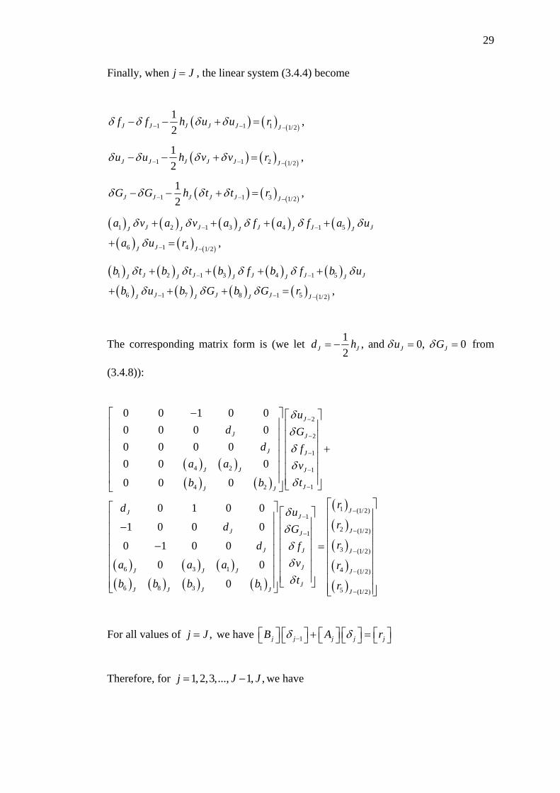
Finally, when j J= , the linear system (3.4.4) become

( ) ( ) ( )1 1 1 1/2

1 ,2J J J J J J

f f h u u rδ δ δ δ− − −− − + =

( ) ( ) ( )1 1 2 1/2

1 ,2J J J J J J

u u h v v rδ δ δ δ− − −− − + =

( ) ( ) ( )1 1 3 1/2

1 ,2J J J J J J

G G h t t rδ δ δ δ− − −− − + =

( ) ( ) ( ) ( ) ( )( ) ( ) ( )

1 2 1 3 4 1 5

6 1 4 1/2,

J J J J JJ J J J J

JJ J

a v a v a f a f a u

a u r

δ δ δ δ δ

δ− −

− −

+ + + +

+ =

( ) ( ) ( ) ( ) ( )( ) ( ) ( ) ( ) ( )

1 2 1 3 4 1 5

6 1 7 8 1 5 1/2,

J J J J JJ J J J J

J J JJ J J J

b t b t b f b f b u

b u b G b G r

δ δ δ δ δ

δ δ δ− −

− − −

+ + + +

+ + + =

The corresponding matrix form is (we let 1 , and 0, 02J J J Jd h u Gδ δ= − = = from

(3.4.8)):

( ) ( )( ) ( )

( ) ( ) ( )( ) ( ) ( ) ( )

( )

2

2

1

4 2 1

14 2

1 (1/21

1

6 3 1

6 8 3 1

0 0 1 0 00 0 0 00 0 0 00 0 0

0 0 0

0 1 0 0

1 0 0 0

0 1 0 0

0 0

0

J

J J

J J

J J J

JJ J

JJ J

J J

J J

JJ J J

JJ J J J

ud G

d fa a v

tb b

rd ud G

d fva a atb b b b

δδδδδ

δδδδδ

−

−

−

−

−

−−

−

−⎡ ⎤ ⎡ ⎤⎢ ⎥ ⎢ ⎥⎢ ⎥ ⎢ ⎥⎢ ⎥ ⎢ ⎥ +⎢ ⎥ ⎢ ⎥⎢ ⎥ ⎢ ⎥⎢ ⎥ ⎢ ⎥⎣ ⎦⎣ ⎦

⎡ ⎤ ⎡ ⎤⎢ ⎥ ⎢ ⎥−⎢ ⎥ ⎢ ⎥⎢ ⎥ ⎢ ⎥− =⎢ ⎥ ⎢ ⎥⎢ ⎥ ⎢ ⎥⎢ ⎥ ⎢ ⎥⎣ ⎦⎢ ⎥⎣ ⎦

( )( )( )( )

)

2 (1/2)

3 (1/2)

4 (1/2)

5 (1/2)

J

J

J

J

r

r

r

r

−

−

−

−

⎡ ⎤⎢ ⎥⎢ ⎥⎢ ⎥⎢ ⎥⎢ ⎥⎢ ⎥⎢ ⎥⎢ ⎥⎣ ⎦

For all values of ,j J= we have 1j j j j jB A rδ δ−⎡ ⎤ ⎡ ⎤ ⎡ ⎤ ⎡ ⎤ ⎡ ⎤+ =⎣ ⎦ ⎣ ⎦ ⎣ ⎦ ⎣ ⎦ ⎣ ⎦

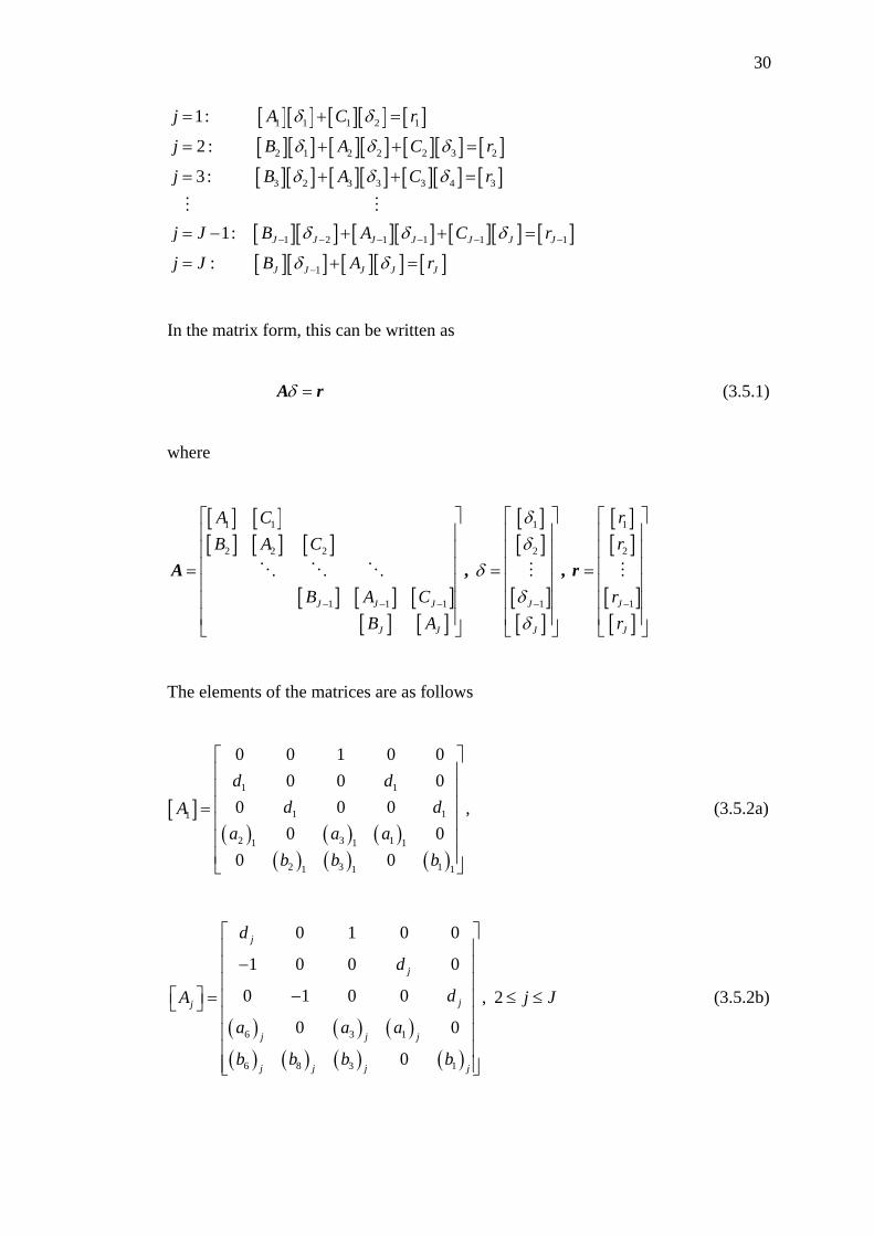
Therefore, for 1,2,3,..., 1, ,j J J= − we have

30

[ ][ ] [ ][ ] [ ][ ][ ] [ ][ ] [ ][ ] [ ][ ][ ] [ ][ ] [ ][ ] [ ]

[ ][ ] [ ][ ] [ ][ ] [ ][ ][ ] [ ]

1 1 1 2 1

2 1 2 2 2 3 2

3 2 3 3 3 4 3

1 2 1 1 1 1

1

1:

2 :

3 :

1:

: J J J J J J J

J J J

j A C r

j B A C r

j B A C r

j J B A C r

j J B A

δ δ

δ δ δ

δ δ δ

δ δ δ

δ δ− − − − − −

−

= + =

= + + =

= + + =

= − + + =

= +

M M

[ ] [ ]J Jr=

In the matrix form, this can be written as

δ =A r (3.5.1)

where

[ ] [ ][ ] [ ] [ ]

[ ] [ ] [ ][ ] [ ]

[ ][ ]

[ ][ ]

[ ][ ]

[ ][ ]

1 1 1 1

2 2 2 2 2

1 1 1 1 1

J J J J J

J J J J

A C rB A C r

B A C rB A r

δδ

δδδ

− − − − −

⎡ ⎤ ⎡ ⎤ ⎡ ⎤⎢ ⎥ ⎢ ⎥ ⎢ ⎥⎢ ⎥ ⎢ ⎥ ⎢ ⎥⎢ ⎥ ⎢ ⎥ ⎢ ⎥= = =⎢ ⎥ ⎢ ⎥ ⎢ ⎥⎢ ⎥ ⎢ ⎥ ⎢ ⎥⎢ ⎥ ⎢ ⎥ ⎢ ⎥⎣ ⎦ ⎣ ⎦ ⎣ ⎦

, ,O O O M MA r

The elements of the matrices are as follows

[ ]( ) ( ) ( )

( ) ( ) ( )

1 1

1 11

2 3 11 1 1

2 3 11 1 1

0 0 1 0 00 0 0

0 0 0 ,0 0

0 0

d dd dA

a a ab b b

⎡ ⎤⎢ ⎥⎢ ⎥⎢ ⎥=⎢ ⎥⎢ ⎥⎢ ⎥⎣ ⎦

(3.5.2a)

( ) ( ) ( )( ) ( ) ( ) ( )

6 3 1

6 8 3 1

0 1 0 0

1 0 0 0

0 1 0 0 , 2

0 0

0

j

j

jj

j j j

j j j j

d

d

dA j J

a a a

b b b b

⎡ ⎤⎢ ⎥−⎢ ⎥

⎢ ⎥−⎡ ⎤ = ≤ ≤⎢ ⎥⎣ ⎦

⎢ ⎥⎢ ⎥⎢ ⎥⎢ ⎥⎣ ⎦

(3.5.2b)

31

( ) ( )( ) ( )

4 2

4 2

0 0 1 0 00 0 0 00 0 0 0 , 20 0 0

0 0 0

j

jj

j j

j j

ddB j J

a a

b b

−⎡ ⎤⎢ ⎥⎢ ⎥⎢ ⎥⎡ ⎤ = ≤ ≤⎣ ⎦ ⎢ ⎥⎢ ⎥⎢ ⎥⎢ ⎥⎣ ⎦

(3.5.3)

( )( ) ( )

5

5 7

0 0 0 0

1 0 0 0 0

0 1 0 0 0 , 1 1

0 0 0 0

0 0 0

j

j

j

j j

d

C j J

a

b b

⎡ ⎤⎢ ⎥⎢ ⎥⎢ ⎥

⎡ ⎤ = ≤ ≤ −⎢ ⎥⎣ ⎦⎢ ⎥⎢ ⎥⎢ ⎥⎢ ⎥⎣ ⎦

(3.5.4)

[ ]

10

10

1 1

1

1

, , 2

j

j

j

j

j

uvGt

f j Jfvvtt

δδδδδδ δδδδδδ

−

−

⎡ ⎤⎡ ⎤⎢ ⎥⎢ ⎥⎢ ⎥⎢ ⎥⎢ ⎥⎢ ⎥= = ≤ ≤⎢ ⎥⎢ ⎥⎢ ⎥⎢ ⎥⎢ ⎥⎢ ⎥⎣ ⎦ ⎣ ⎦

(3.5.5a, b)

And

( )( )( )( )( )

1 (1/2)

2 (1/2)

3 (1/2)

4 (1/2)

5 (1/2)

, 1

j

j

j j

j

j

r

r

rr j J

r

r

−

−

−

−

−

⎡ ⎤⎢ ⎥⎢ ⎥⎢ ⎥

⎡ ⎤ = ≤ ≤⎢ ⎥⎣ ⎦⎢ ⎥⎢ ⎥⎢ ⎥⎢ ⎥⎣ ⎦

(3.5.6)

The coefficient matrix A is known as tridiagonal matrix due to the fact that

all elements of A are zero except those on the three main diagonal. To solve

equation (3.5.1), according to the block elimination method as described in Cebeci

and Bradshaw (1988), we assume matrix A is nonsingular and we seek a

factorization of the form

=A LU (3.5.7)

where

32

[ ][ ] [ ]

[ ] [ ]

[ ] [ ][ ] [ ]

1

2 2

3 3

1 1J J

J J

BB

BB

αα

α

αα

− −

⎡ ⎤⎢ ⎥⎢ ⎥⎢ ⎥⎢ ⎥

= ⎢ ⎥⎢ ⎥⎢ ⎥⎢ ⎥⎢ ⎥⎣ ⎦

O

O

L

and

[ ] [ ][ ] [ ]

[ ] [ ]

[ ] [ ][ ]

1

2

3

1J

II

I

II−

⎡ ⎤Γ⎢ ⎥Γ⎢ ⎥⎢ ⎥Γ⎢ ⎥

= ⎢ ⎥⎢ ⎥⎢ ⎥

Γ⎢ ⎥⎢ ⎥⎣ ⎦

,O

O

U

[ ]I is the identity matrix of order 5. [ ]iα and [ ]iΓ are 5 x 5 matrices whose element

are determined by the following equations:

[ ] [ ]1 1Aα = , (3.5.8a)

[ ][ ] [ ]1 1 1A CΓ = (3.5.8b)

and

1 2 3j j j jA B j Jα −⎡ ⎤ ⎡ ⎤ ⎡ ⎤ ⎡ ⎤= − Γ =⎣ ⎦ ⎣ ⎦ ⎣ ⎦ ⎣ ⎦ , , , ,K (3.5.8c)

2 3 1j j jC j Jα⎡ ⎤ ⎡ ⎤ ⎡ ⎤Γ = = −⎣ ⎦ ⎣ ⎦ ⎣ ⎦ , , , , .K (3.5.8d)

By substituting (3.5.7) into (3.5.1), we get

δ =LU r (3.5.9)

If we define δ =U W (3.5.10)

33

then equation (3.5.9) becomes =LW r (3.5.11)

where

[ ][ ]

[ ][ ]

1

2

1J

J

WW

WW

−

⎡ ⎤⎢ ⎥⎢ ⎥⎢ ⎥=⎢ ⎥⎢ ⎥⎢ ⎥⎣ ⎦

,MW

and jW⎡ ⎤⎣ ⎦ are 5 x 1 column matrices. The elements W can be solved from equation

(3.5.11):

[ ][ ] [ ]1 1 1W rα = , (3.5.12a)

1 2j j j j jW r B W j Jα −⎡ ⎤ ⎡ ⎤ ⎡ ⎤ ⎡ ⎤ ⎡ ⎤= − ≤ ≤⎣ ⎦ ⎣ ⎦ ⎣ ⎦ ⎣ ⎦ ⎣ ⎦ , (3.5.12b)

The solution of equation (3.5.7) by block-elimination method consists of two

sweeps. The step in which and j j jWαΓ , are calculated, is usually referred to as the

forward sweep. They are computed from the recursion formulas given by (3.5.8) and

(3.5.12). When the elements of W are found, equation (3.5.10) then gives the solution

of δ in the so called backward sweep, in which the elements are obtained by the

following relations:

[ ] [ ]J JWδ = , (3.5.13a)

1 1 1j j j jW j Jδ δ +⎡ ⎤ ⎡ ⎤ ⎡ ⎤ ⎡ ⎤= − Γ ≤ ≤ −⎣ ⎦ ⎣ ⎦ ⎣ ⎦ ⎣ ⎦ , (3.5.13b)

Once the elements of δ are found, equation (3.4.4) can be used to find (i+1)th

iteration in equation (3.4.3).

These calculations are repeated until some convergence criterion is satisfied.

In laminar boundary layer calculations, the wall shear stress parameter ( )0,v x is

34

usually used as the convergence criterion. This is probably because in boundary layer

calculations, it is find that the greatest error usually appears in the wall shear stress

parameter. Calculations are stopped when

( )0 1ivδ ε< (3.5.14)

where 1ε is a small prescribed value.

In this study, we consider 51 10ε −= that gives about four decimal places

accuracy for most predicted quantities (Cebeci and Bradshaw (1988)).

3.6 Starting Conditions

In the numerical computation, a proper step size yΔ and an appropriate

y∞ value (an approximate to y = ∞ ) must be determined. All of these value usually

determined by a trial and error approach (Chen (1998)). In general, if the appropriate

y∞ value at a given x is not known, the computation can be started by using small

value of y∞ and the successively increase the values of y∞ until a suitable y∞ is

obtained.

For most laminar boundary layer flows the transformed boundary layer

thickness ( )y x∞ is almost constant. The value of y∞ typically lies between 5 and 10.

Once we obtain the proper values of y∞ , a reasonable choice of step size yΔ and

xΔ should be determined. In most laminar boundary layer flows, a step size

0 02.yΔ = to 0.04 is sufficient to provide accurate and comparable results.

In order to start and proceed with the numerical computation, it is necessary

to make initial guesses for the function and , , ,f u v G t across the boundary layer. To

start a solution at a given x, it is necessary to assume distribution curves for the

35

velocity, u and the temperature, G between 0y = and y y∞= . We used the

distribution curves given by Bejan (1984) and Ghoshdastidar (2004). These are used

as the initial guess because both the velocity and temperature profiles satisfy the

boundary condition for the problem of heat transfer characteristic of a continuous

stretching surface with thermal boundary condition for uniform and variable surface

temperature.

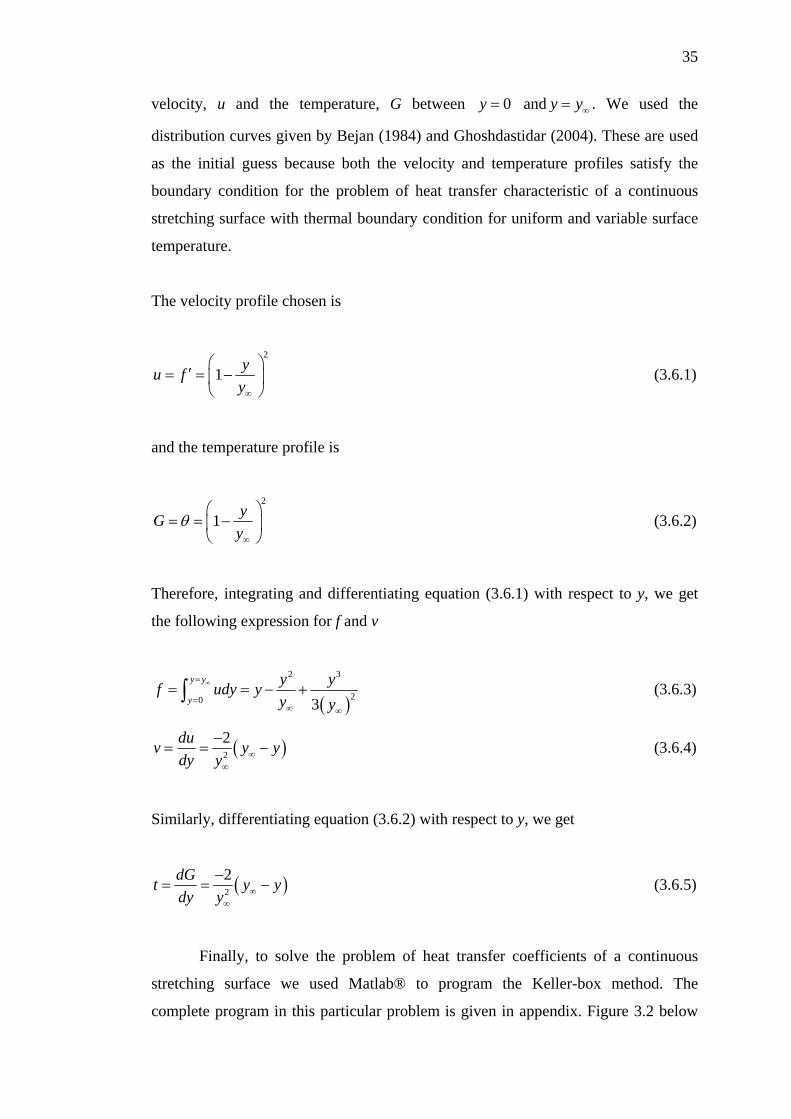
The velocity profile chosen is

2

1 yu fy∞

⎛ ⎞′= = −⎜ ⎟

⎝ ⎠ (3.6.1)

and the temperature profile is

2

1 yGy

θ∞

⎛ ⎞= = −⎜ ⎟

⎝ ⎠ (3.6.2)

Therefore, integrating and differentiating equation (3.6.1) with respect to y, we get

the following expression for f and v

( )

2 3

20 3

y y

y

y yf udy yy y

∞=

=∞ ∞

= = − +∫ (3.6.3)

( )2

2duv y ydy y ∞

∞

−= = − (3.6.4)

Similarly, differentiating equation (3.6.2) with respect to y, we get

( )2

2dGt y ydy y ∞

∞

−= = − (3.6.5)

Finally, to solve the problem of heat transfer coefficients of a continuous

stretching surface we used Matlab® to program the Keller-box method. The

complete program in this particular problem is given in appendix. Figure 3.2 below

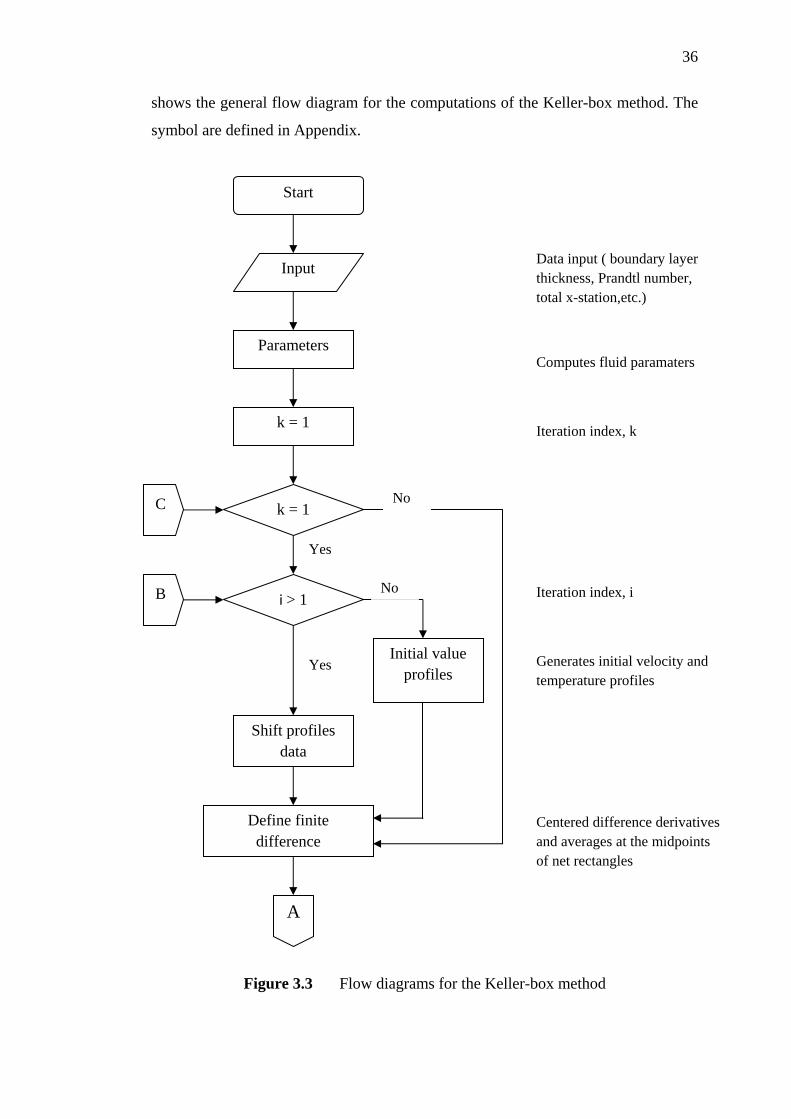
36

shows the general flow diagram for the computations of the Keller-box method. The

symbol are defined in Appendix.

Figure 3.3 Flow diagrams for the Keller-box method

A

Define finite difference

Shift profiles data

C

B i > 1

Initial value profiles

Parameters

k = 1

k = 1

Start

Input

No

Yes

No

Yes

Data input ( boundary layer thickness, Prandtl number, total x-station,etc.)

Computes fluid paramaters

Iteration index, k

Iteration index, i

Generates initial velocity and temperature profiles

Centered difference derivatives and averages at the midpoints of net rectangles

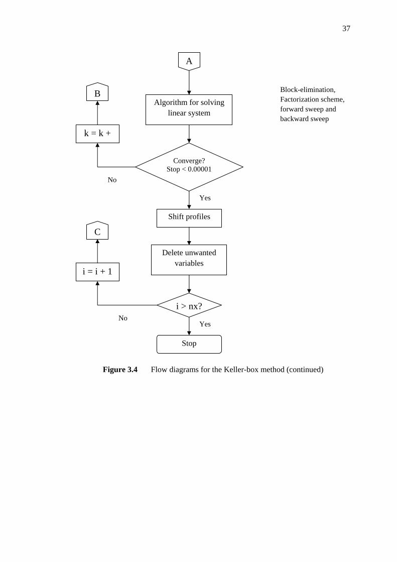
37

Figure 3.4 Flow diagrams for the Keller-box method (continued)

Stop

i > nx?

Shift profiles

Delete unwanted variables

Algorithm for solving linear system

Converge? Stop < 0.00001

A

B

k = k +

C

i = i + 1

Yes

No

YesNo

Block-elimination, Factorization scheme, forward sweep and backward sweep

CHAPTER IV

HEAT TRANSFER COEFFICIENTS ON A CONTINOUOUS STRECTHING SURFACE

4.1 Introduction

In this chapter, the problem of heat transfer coefficients on a continuous

stretching surface is considered and discussed. We will use the Keller-box method

that has been described in Chapter 3 to solve this problem. Three cases of thermal

boundary conditions, namely uniform surface temperature ( )0n = , variable surface

temperature ( )0n ≠ and uniform heat flux ( )( )1 2n m= − are presented in the

following three main section.

Section 4.2 will discuss the problem of heat transfer stretching surface with

uniform surface temperature conditions and the result will be discussed in Section

4.2.1. The ordinary differential equations for problem with variable surface

temperature are given in Section 4.3 and in Section 4.3.1 the result for this problem

will be discussed. In the last section, Section 4.4 the problem for thermal boundary

condition with uniform heat flux will be discussed and the results are presented in

section 4.4.1.

39

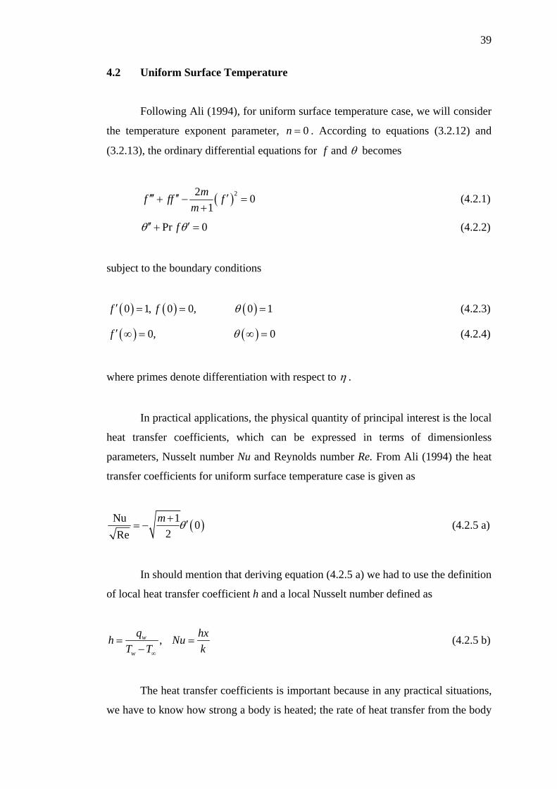
4.2 Uniform Surface Temperature Following Ali (1994), for uniform surface temperature case, we will consider

the temperature exponent parameter, 0n = . According to equations (3.2.12) and

(3.2.13), the ordinary differential equations for f and θ becomes

( )22 01

mf ff fm

′′′ ′′ ′+ − =+

(4.2.1)

Pr 0fθ θ′′ ′+ = (4.2.2)

subject to the boundary conditions

( ) ( ) ( )0 1, 0 0, 0 1f f θ′ = = = (4.2.3)

( ) ( )0, 0f θ′ ∞ = ∞ = (4.2.4)

where primes denote differentiation with respect to η .

In practical applications, the physical quantity of principal interest is the local

heat transfer coefficients, which can be expressed in terms of dimensionless

parameters, Nusselt number Nu and Reynolds number Re. From Ali (1994) the heat

transfer coefficients for uniform surface temperature case is given as

( )Nu 1 02Re

m θ+ ′= − (4.2.5 a)

In should mention that deriving equation (4.2.5 a) we had to use the definition

of local heat transfer coefficient h and a local Nusselt number defined as

, w

w

q hxh NuT T k∞

= =−

(4.2.5 b)

The heat transfer coefficients is important because in any practical situations,

we have to know how strong a body is heated; the rate of heat transfer from the body

40

to the fluid; what kind of materials we have to use in order to avoid the body to be

exposed to high temperatures, etc. All the practical devices that operate with the use

of heat are designed based on theoretical or experimental heat transfer coefficients,

such as nuclear devices, insulation of buildings.

4.2.1 Results and Discussion

Equation (4.2.1) and (4.2.2) subject to boundary conditions (4.2.3) and (4.2.4)

were solved using the Keller-box. The solution procedure using this method has been

discussed in Chapter III. All the results quoted here were obtained using uniform grid

in η direction. We used the step size of 0.05ηΔ = . In all cases we choose 10η = .

The initial profiles for this problem are given by equations (3.6.1) to (3.6.5).

Details results are for temperature profiles, ( )θ η and heat transfer

coefficient, ReNu are obtained for the following values of velocity exponent

parameter, 0 41 3. m− ≤ ≤ and 3 1 1m .− ≤ ≤ − with Prandtl number, Pr = 0.72, 1.0, 3.0

and 10. In order to access the accuracy of the present method, we have compared the

results for the heat transfer coefficient, ReNu for 0 and 0m n= = and

temperature gradient ( )0θ ′ for 1m = and 0n = with previously published result and

found them into excellent agreement. The comparison is shown in Table 4.1 and

Table 4.2. This favorable comparison lends confidence in the numerical results

obtain in this paper.

Table 4.1: Heat transfer coefficient NuRe

for 0 and 0m n= = .

Pr

Jacobi (1993)

Soundalgekar and Murty (1980)

Chen (1980)

Tsou et al (1967)

Ali (1994)

Present

0.7 0.3492 0.3508 0.3492 0.3492 0.3476 0.3493 1.0 0.4438 - - 0.4438 0.4416 0.4438 10.0 1.6790 1.6808 - 1.6804 1.6713 1.6804

41

Table 4.2: Temperature gradient ( )0θ ′ for 1 and 0m n= = .

Pr Grubka and Bobba (1985)

Lakshmisha et al (1988)

Gupta (1977)

Ali (1994)

Present

0.7 - 0.45446 - -0.45255 -0.4540 1.0 -0.5820 - -0.5820 -0.59988 -0.5820 10.0 -2.3080 - - -2.29589 -2.3082 1.0 - - -0.1105 -0.10996 -0.1106

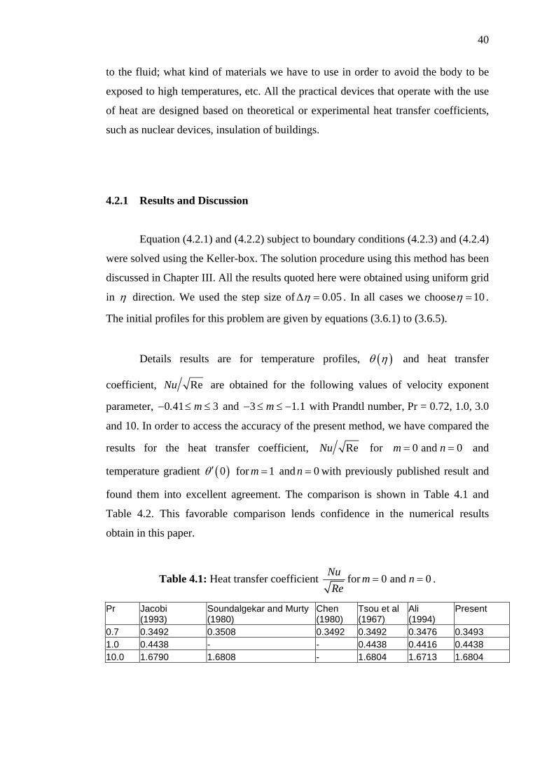
Figure 4.1 to 4.3 illustrate the dimensionless temperature profiles, ( )θ η and

heat transfer coefficient, ReNu for various values of Prandtl numbers and

velocity. Figure 4.1 shows that when 3 and 0m n= = the thermal boundary layer

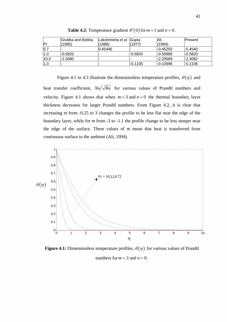
thickness decreases for larger Prandtl numbers. From Figure 4.2, it is clear that

increasing m from -0.25 to 3 changes the profile to be less flat near the edge of the

boundary layer, while for m from -3 to -1.1 the profile change to be less steeper near

the edge of the surface. These values of m mean that heat is transferred from

continuous surface to the ambient (Ali, 1994).

Figure 4.1: Dimensionless temperature profiles, ( )θ η for various values of Prandtl

numbers for 3 and 0m n= = .

0 1 2 3 4 5 6 7 8 9 100

0.1

0.2

0.3

0.4

0.5

0.6

0.7

0.8

0.9

1

η

Pr = 10,3,1,0.72

( )θ η

42

Figure 4.2: Dimensionless temperature profiles, ( )θ η for various values of m

for 0 and Pr 0.72n = = .

Figure 4.3 presented the heat transfer coefficient in the dimensionless form of

ReNu as a function of m in the range of 0 41 3. m− ≤ ≤ for different Prandtl

numbers. It shows that the increasing velocity exponent parameters, m and Prandtl

number enhance the heat transfer coefficient, ReNu . Moreover, increasing

Prandtl number increases the rate of heat transfer coefficient, ReNu .

0 1 2 3 4 5 6 7 8 9 100

0.2

0.4

0.6

0.8

1

η

m = -3.0

m = -1.1

m = -0.25

m = 0.0

m = 3.0

( )θ η

43

enhance the heat transfer coefficient. Moreover, increasing Prandtl number also

increase the rate of heat transfer coefficie

Figure 4.3: Variation of NuRe

as a function of m at n = 0 and for different values of

Prandtl number.

4.3 Variable Surface Temperature

In this section we will consider the variable surface temperature case ( )0n ≠ .

According to equations (3.2.12) and (3.2.13), the ordinary differential equations for

f and θ becomes

( )22 01

mf ff fm

′′′ ′′ ′+ − =+

(3.2.12)

2Pr 01

nf fm

θ θ θ⎡ ⎤′′ ′ ′+ − =⎢ ⎥+⎣ ⎦ (3.2.13)

subject to

( ) ( ) ( )0 1, 0 0, 0 1f f θ′ = = = (3.2.14)

( ) ( )0, 0f θ′ ∞ = ∞ = (3.2.15)

-1 -0.5 0 0.5 1 1.5 2 2.5 3 3.50

0.5

1

1.5

2

2.5

3

3.5

m

Pr = 0.72,1.0,3.0,10

NuRe

m

44

where primes denote differentiation with respect to η .

In practical applications, the physical quantities of principal interest are the

local heat transfer coefficients are same with the uniform surface temperature case.


Equation (3.2.12) and (3.2.13) subject to boundary conditions (3.2.14) and

(3.2.15) were solved using the Keller-box. The solution procedure using this method

has been discussed in Chapter III. All the results quoted here were obtained using

uniform grid in η direction. We used the step size of 0.05ηΔ = . In all cases we

choose 10η = . The initial profiles for this problem are given by equations (3.6.1) -

(3.6.5).

Details results are for temperature profiles, ( )θ η and heat transfer coefficient,

ReNu are obtained for the following values of velocity exponent parameter,

0 41 3. m− ≤ ≤ and 3 1 1m .− ≤ ≤ − and temperature exponent parameter, 0n ≠ with

Prandtl number, Pr = 0.72, 1.0, 3.0 and 10. The accuracy of this numerical method

was validated by direct comparison with the numerical results reported earlier by

Chen (1998), Grubka and Bobba (1985) and Ishak et al (2007) for 1m = . Table 4.3

present the temperature gradient, ( )0θ ′ , it can be seen from Table 4.3 that very good

agreement between the results exists. This favorable comparison lends confidence in

the numerical results obtained in this paper.

Table 4.3: Temperature gradient ( )0θ ′ for 1m = .

Grubka and Bobba

(1985) Ishak et al

(2007) Present

n Pr = 1 Pr = 3 Pr = 10 Pr = 1 Pr = 3 Pr = 10 Pr = 1 Pr = 3 Pr = 10-2 1.0000 3.0000 10.0000 1.0000 3.0000 10.0000 0.9994 2.9999 9.9988-1 0.0000 0.0000 0.0000 0.0000 0.0000 0.0000 -0.0001 0.0000 0.00000 -0.5820 -1.1652 -2.3080 -0.5820 -1.1652 -2.3080 -0.5820 -1.1653 -2.30811 -1.0000 -1.9237 -3.7207 -1.0000 -1.9237 -3.7207 -1.0000 -1.9237 -3.72082 -1.3333 -2.5097 -4.7969 -1.3333 -2.5097 -4.7969 -1.3333 -2.5097 -4.7970

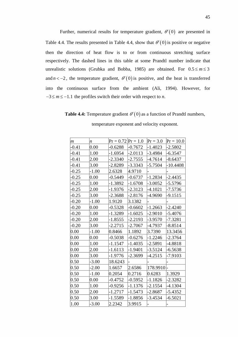
45

Further, numerical results for temperature gradient, ( )0θ ′ are presented in

Table 4.4. The results presented in Table 4.4, show that ( )0θ ′ is positive or negative

then the direction of heat flow is to or from continuous stretching surface

respectively. The dashed lines in this table at some Prandtl number indicate that

unrealistic solutions (Grubka and Bobba, 1985) are obtained. For 0.5 3m≤ ≤

and 2n < − , the temperature gradient, ( )0θ ′ is positive, and the heat is transferred

into the continuous surface from the ambient (Ali, 1994). However, for

3 1 1m .− ≤ ≤ − the profiles switch their order with respect to n.

Table 4.4: Temperature gradient ( )0θ ′ as a function of Prandtl numbers,

temperature exponent and velocity exponent.

m n Pr = 0.72 Pr = 1.0 Pr = 3.0 Pr = 10.0 -0.41 0.00 -0.6288 -0.7672 -1.4023 -2.5802 -0.41 1.00 -1.6954 -2.0113 -3.4984 -6.3547 -0.41 2.00 -2.3340 -2.7555 -4.7614 -8.6437 -0.41 3.00 -2.8289 -3.3343 -5.7504 -10.4408 -0.25 -1.00 2.6328 4.9710 - - -0.25 0.00 -0.5449 -0.6737 -1.2834 -2.4435 -0.25 1.00 -1.3892 -1.6708 -3.0052 -5.5796 -0.25 2.00 -1.9376 -2.3123 -4.1021 -7.5736 -0.25 3.00 -2.3688 -2.8176 -4.9690 -9.1515 -0.20 -1.00 1.9120 3.1382 - - -0.20 0.00 -0.5328 -0.6602 -1.2663 -2.4240 -0.20 1.00 -1.3289 -1.6025 -2.9010 -5.4076 -0.20 2.00 -1.8555 -2.2193 -3.9570 -7.3281 -0.20 3.00 -2.2715 -2.7067 -4.7937 -8.8514 0.00 -1.00 0.8466 1.1892 3.7390 13.3456 0.00 0.00 -0.5038 -0.6276 -1.2246 -2.3764 0.00 1.00 -1.1547 -1.4035 -2.5891 -4.8818 0.00 2.00 -1.6113 -1.9401 -3.5124 -6.5638 0.00 3.00 -1.9776 -2.3699 -4.2515 -7.9103 0.50 -3.00 18.6243 - - - 0.50 -2.00 1.6657 2.6586 178.9910 - 0.50 -1.00 0.2054 0.2716 0.6283 1.3929 0.50 0.00 -0.4752 -0.5952 -1.1826 -2.3282 0.50 1.00 -0.9256 -1.1376 -2.1554 -4.1304 0.50 2.00 -1.2717 -1.5473 -2.8687 -5.4352 0.50 3.00 -1.5589 -1.8856 -3.4534 -6.5021 1.00 -3.00 2.2342 3.9915 - -

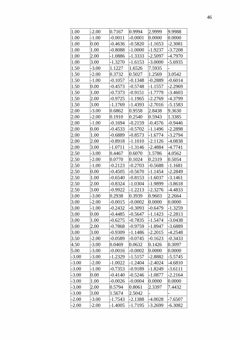
46

1.00 -2.00 0.7167 0.9994 2.9999 9.9988 1.00 -1.00 -0.0011 -0.0001 0.0000 0.0000 1.00 0.00 -0.4636 -0.5820 -1.1653 -2.3081 1.00 1.00 -0.8088 -1.0000 -1.9237 -3.7208 1.00 2.00 -1.0886 -1.3333 -2.5097 -4.7970 1.00 3.00 -1.3270 -1.6153 -3.0000 -5.6935 1.50 -3.00 1.1227 1.6526 7.5935 - 1.50 -2.00 0.3732 0.5027 1.2569 3.0542 1.50 -1.00 -0.1057 -0.1348 -0.2889 -0.6014 1.50 0.00 -0.4573 -0.5748 -1.1557 -2.2969 1.50 1.00 -0.7373 -0.9151 -1.7779 -3.4603 1.50 2.00 -0.9725 -1.1965 -2.2769 -4.3799 1.50 3.00 -1.1769 -1.4393 -2.7016 -5.1583 2.00 -3.00 0.6862 0.9558 2.8438 9.3630 2.00 -2.00 0.1910 0.2540 0.5943 1.3385 2.00 -1.00 -0.1694 -0.2159 -0.4576 -0.9446 2.00 0.00 -0.4533 -0.5702 -1.1496 -2.2898 2.00 1.00 -0.6889 -0.8573 -1.6774 -3.2794 2.00 2.00 -0.8918 -1.1010 -2.1126 -4.0838 2.00 3.00 -1.0711 -1.3146 -2.4884 -4.7741 2.50 -3.00 0.4467 0.6070 1.5786 4.0562 2.50 -2.00 0.0770 0.1024 0.2319 0.5054 2.50 -1.00 -0.2123 -0.2703 -0.5688 -1.1681 2.50 0.00 -0.4505 -0.5670 -1.1454 -2.2849 2.50 1.00 -0.6540 -0.8153 -1.6037 -3.1461 2.50 2.00 -0.8324 -1.0304 -1.9899 -3.8618 2.50 3.00 -0.9922 -1.2213 -2.3276 -4.4833 3.00 -3.00 0.2938 0.3939 0.9603 2.2664 3.00 -2.00 -0.0015 -0.0002 0.0000 0.0000 3.00 -1.00 -0.2432 -0.3093 -0.6479 -1.3259 3.00 0.00 -0.4485 -0.5647 -1.1423 -2.2813 3.00 1.00 -0.6275 -0.7835 -1.5474 -3.0438 3.00 2.00 -0.7868 -0.9759 -1.8947 -3.6889 3.00 3.00 -0.9309 -1.1486 -2.2015 -4.2548 3.50 -2.00 -0.0589 -0.0745 -0.1623 -0.3433 4.50 -3.00 0.0469 0.0632 0.1426 0.3097 5.00 -3.00 -0.0016 -0.0002 0.0000 0.0000 -3.00 -3.00 -1.2329 -1.5157 -2.8882 -5.5745 -3.00 -2.00 -1.0022 -1.2404 -2.4024 -4.6810 -3.00 -1.00 -0.7353 -0.9189 -1.8249 -3.6111 -3.00 0.00 -0.4140 -0.5246 -1.0877 -2.2164 -3.00 1.00 -0.0026 -0.0004 0.0000 0.0000 -3.00 2.00 0.5794 0.8061 2.3397 7.4432 -3.00 3.00 1.5674 2.5042 - - -2.00 -3.00 -1.7543 -2.1388 -4.0028 -7.6507 -2.00 -2.00 -1.4005 -1.7195 -3.2699 -6.3082

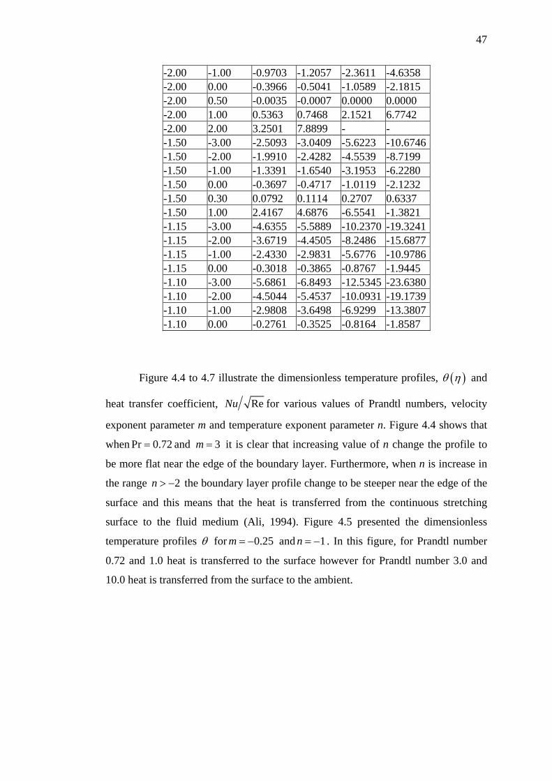
47

-2.00 -1.00 -0.9703 -1.2057 -2.3611 -4.6358 -2.00 0.00 -0.3966 -0.5041 -1.0589 -2.1815 -2.00 0.50 -0.0035 -0.0007 0.0000 0.0000 -2.00 1.00 0.5363 0.7468 2.1521 6.7742 -2.00 2.00 3.2501 7.8899 - - -1.50 -3.00 -2.5093 -3.0409 -5.6223 -10.6746 -1.50 -2.00 -1.9910 -2.4282 -4.5539 -8.7199 -1.50 -1.00 -1.3391 -1.6540 -3.1953 -6.2280 -1.50 0.00 -0.3697 -0.4717 -1.0119 -2.1232 -1.50 0.30 0.0792 0.1114 0.2707 0.6337 -1.50 1.00 2.4167 4.6876 -6.5541 -1.3821 -1.15 -3.00 -4.6355 -5.5889 -10.2370 -19.3241 -1.15 -2.00 -3.6719 -4.4505 -8.2486 -15.6877 -1.15 -1.00 -2.4330 -2.9831 -5.6776 -10.9786 -1.15 0.00 -0.3018 -0.3865 -0.8767 -1.9445 -1.10 -3.00 -5.6861 -6.8493 -12.5345 -23.6380 -1.10 -2.00 -4.5044 -5.4537 -10.0931 -19.1739 -1.10 -1.00 -2.9808 -3.6498 -6.9299 -13.3807 -1.10 0.00 -0.2761 -0.3525 -0.8164 -1.8587

Figure 4.4 to 4.7 illustrate the dimensionless temperature profiles, ( )θ η and

heat transfer coefficient, ReNu for various values of Prandtl numbers, velocity

exponent parameter m and temperature exponent parameter n. Figure 4.4 shows that

when Pr 0.72= and 3m = it is clear that increasing value of n change the profile to

be more flat near the edge of the boundary layer. Furthermore, when n is increase in

the range 2n > − the boundary layer profile change to be steeper near the edge of the

surface and this means that the heat is transferred from the continuous stretching

surface to the fluid medium (Ali, 1994). Figure 4.5 presented the dimensionless

temperature profiles θ for 0.25m = − and 1n = − . In this figure, for Prandtl number

0.72 and 1.0 heat is transferred to the surface however for Prandtl number 3.0 and

10.0 heat is transferred from the surface to the ambient.

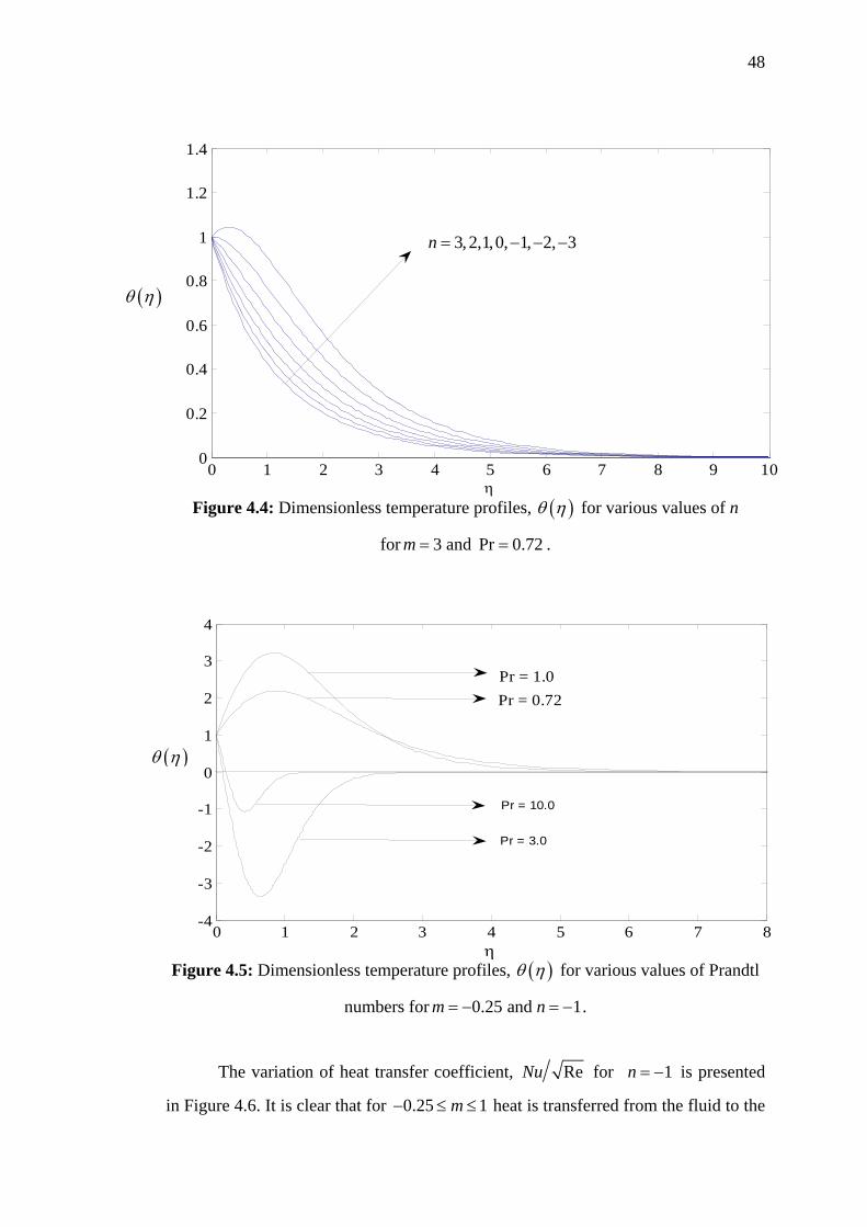
48

Figure 4.4: Dimensionless temperature profiles, ( )θ η for various values of n

for 3 and Pr 0.72m = = .


numbers for 0.25 and 1m n= − = − .

The variation of heat transfer coefficient, ReNu for 1n = − is presented

in Figure 4.6. It is clear that for 0.25 1m− ≤ ≤ heat is transferred from the fluid to the

0 1 2 3 4 5 6 7 8-4

-3

-2

-1

0

1

2

3

4

η

Pr = 1.0Pr = 0.72

Pr = 10.0

Pr = 3.0

( )θ η

0 1 2 3 4 5 6 7 8 9 100

0.2

0.4

0.6

0.8

1

1.2

1.4

η

n = 3,2, 1,0,-1,-2,-3

( )θ η

3, 2,1,0, 1, 2, 3n = − − −

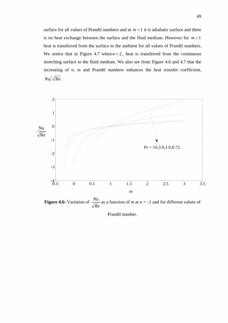
49

surface for all values of Prandtl numbers and at 1m = it is adiabatic surface and there

is no heat exchange between the surface and the fluid medium. However for 1m >

heat is transferred from the surface to the ambient for all values of Prandtl numbers.

We notice that in Figure 4.7 when 2n = , heat is transferred from the continuous

stretching surface to the fluid medium. We also see from Figure 4.6 and 4.7 that the

increasing of n, m and Prandtl numbers enhances the heat transfer coefficient,

ReNu .


as a function of m at n = -1 and for different values of

Prandtl number.

-0.5 0 0.5 1 1.5 2 2.5 3 3.5-4

-3

-2

-1

0

1

2

m

Pr = 10,3.0,1.0,0.72

NuRe

m

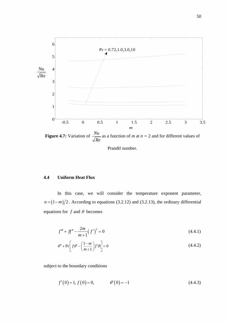
50


as a function of m at n = 2 and for different values of

Prandtl number.

4.4 Uniform Heat Flux

In this case, we will consider the temperature exponent parameter,

( )1 2n m= − . According to equations (3.2.12) and (3.2.13), the ordinary differential

equations for f and θ becomes

( )22 01

mf ff fm

′′′ ′′ ′+ − =+

(4.4.1)

1Pr 01

mf fm

θ θ θ⎡ ⎤−⎛ ⎞′′ ′ ′+ − =⎜ ⎟⎢ ⎥+⎝ ⎠⎣ ⎦ (4.4.2)

subject to the boundary conditions

( ) ( ) ( )0 1, 0 0, 0 1f f θ′ ′= = = − (4.4.3)

-0.5 0 0.5 1 1.5 2 2.5 3 3.50

1

2

3

4

5

6

m

Pr = 0.72,1.0,3.0,10

NuRe

m

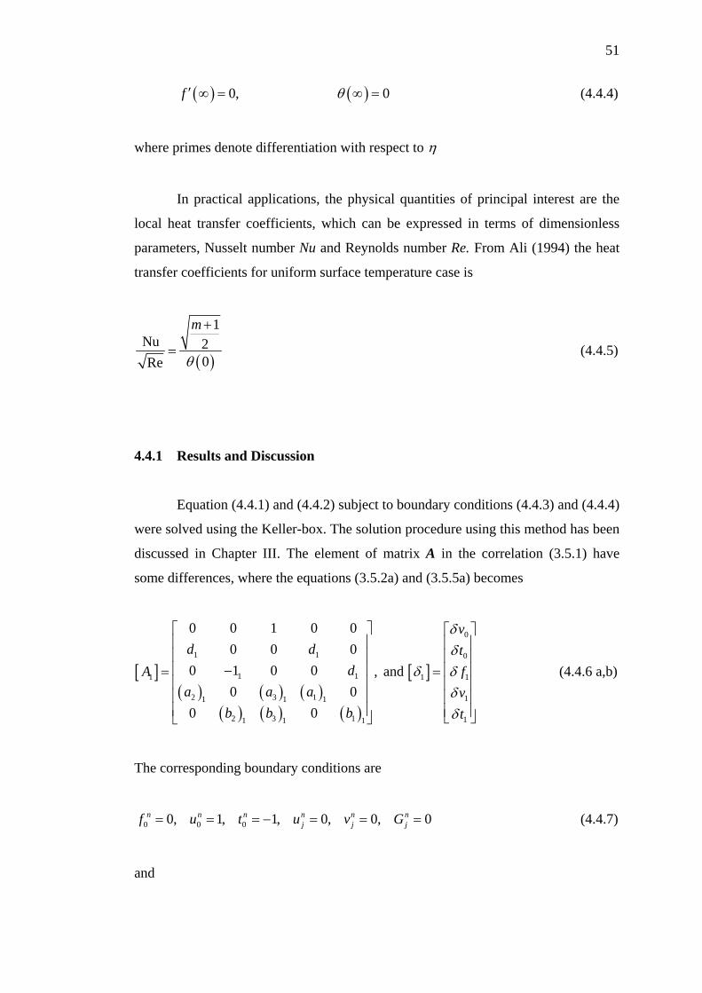
51

( ) ( )0, 0f θ′ ∞ = ∞ = (4.4.4)

where primes denote differentiation with respect to η

In practical applications, the physical quantities of principal interest are the

local heat transfer coefficients, which can be expressed in terms of dimensionless

parameters, Nusselt number Nu and Reynolds number Re. From Ali (1994) the heat

transfer coefficients for uniform surface temperature case is

( )

1Nu 2

0Re

m

θ

+

= (4.4.5)


Equation (4.4.1) and (4.4.2) subject to boundary conditions (4.4.3) and (4.4.4)

were solved using the Keller-box. The solution procedure using this method has been

discussed in Chapter III. The element of matrix A in the correlation (3.5.1) have

some differences, where the equations (3.5.2a) and (3.5.5a) becomes

[ ]( ) ( ) ( )

( ) ( ) ( )

1 1

1 11

2 3 11 1 1

2 3 11 1 1

0 0 1 0 00 0 0

0 1 0 0 ,0 0

0 0

d ddA

a a ab b b

⎡ ⎤⎢ ⎥⎢ ⎥⎢ ⎥−=⎢ ⎥⎢ ⎥⎢ ⎥⎣ ⎦

and [ ]

0

0

1 1

1

1

vtfvt

δδ

δ δδδ

⎡ ⎤⎢ ⎥⎢ ⎥⎢ ⎥=⎢ ⎥⎢ ⎥⎢ ⎥⎣ ⎦

(4.4.6 a,b)

The corresponding boundary conditions are

0 0 00, 1, 1, 0, 0, 0n n n n n nj j jf u t u v G= = = − = = = (4.4.7)

and

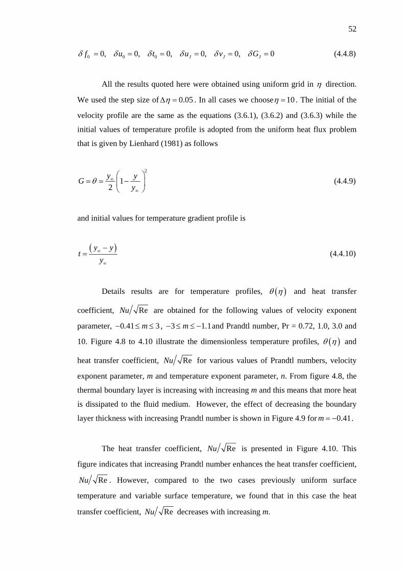
52

0 0 00, 0, 0, 0, 0, 0J J Jf u t u v Gδ δ δ δ δ δ= = = = = = (4.4.8)

All the results quoted here were obtained using uniform grid in η direction.

We used the step size of 0.05ηΔ = . In all cases we choose 10η = . The initial of the

velocity profile are the same as the equations (3.6.1), (3.6.2) and (3.6.3) while the

initial values of temperature profile is adopted from the uniform heat flux problem

that is given by Lienhard (1981) as follows

2

12y yG

yθ ∞

∞

⎛ ⎞= = −⎜ ⎟

⎝ ⎠ (4.4.9)

and initial values for temperature gradient profile is

( )y yt

y∞

∞

−= (4.4.10)

Details results are for temperature profiles, ( )θ η and heat transfer

coefficient, ReNu are obtained for the following values of velocity exponent

parameter, 0 41 3. m− ≤ ≤ , 3 1 1m .− ≤ ≤ − and Prandtl number, Pr = 0.72, 1.0, 3.0 and

10. Figure 4.8 to 4.10 illustrate the dimensionless temperature profiles, ( )θ η and

heat transfer coefficient, ReNu for various values of Prandtl numbers, velocity

exponent parameter, m and temperature exponent parameter, n. From figure 4.8, the

thermal boundary layer is increasing with increasing m and this means that more heat

is dissipated to the fluid medium. However, the effect of decreasing the boundary

layer thickness with increasing Prandtl number is shown in Figure 4.9 for 0.41m = − .

The heat transfer coefficient, ReNu is presented in Figure 4.10. This

figure indicates that increasing Prandtl number enhances the heat transfer coefficient,

ReNu . However, compared to the two cases previously uniform surface

temperature and variable surface temperature, we found that in this case the heat

transfer coefficient, ReNu decreases with increasing m.

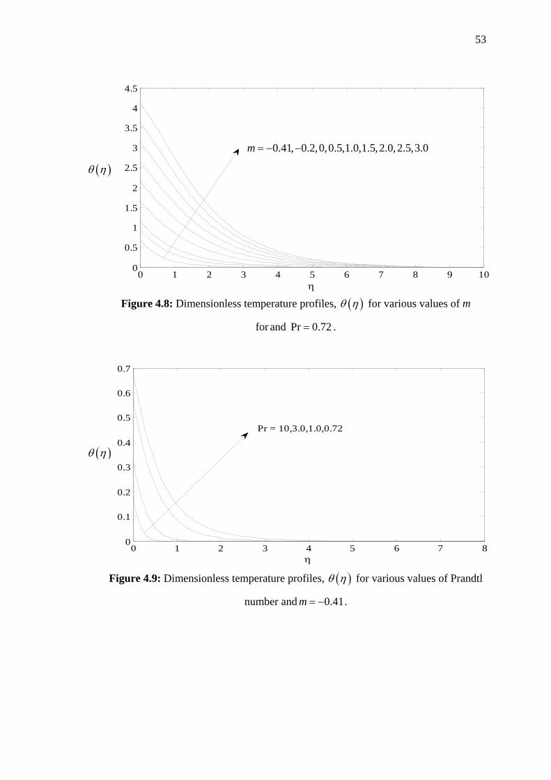
53

Figure 4.8: Dimensionless temperature profiles, ( )θ η for various values of m

for and Pr 0.72= .


number and 0.41m = − .

0 1 2 3 4 5 6 7 80

0.1

0.2

0.3

0.4

0.5

0.6

0.7

η

Pr = 10,3.0,1.0,0.72

( )θ η

0 1 2 3 4 5 6 7 8 9 100

0.5

1

1.5

2

2.5

3

3.5

4

4.5

η

m = -0.41,-0.2,0,0.5,1.0,1.5,2.0,2.5,3.0

( )θ η

0.41, 0.2,0,0.5,1.0,1.5,2.0,2.5,3.0m = − −

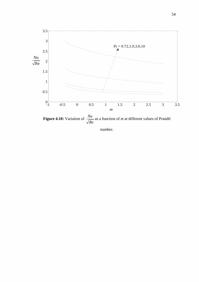
54


as a function of m at different values of Prandtl

number.

-1 -0.5 0 0.5 1 1.5 2 2.5 3 3.50

0.5

1

1.5

2

2.5

3

3.5

m

Pr = 0.72,1.0,3.0,10

NuRe

m

CHAPTER V

g-JITTER FREE CONVECTION ADJACENT TO A VERTICAL STRECHING SHEET

5.1 Introduction

In this chapter, the problem of g-jitter free convection adjacent to vertical

stretching sheet is considered and discussed. We will also use the Keller-box method

that has been described in Chapter 3 to solve this problem. Section 5.2 will discuss

the basic equations of the problem. Finally, in Section 5.3 the result for this problem

will be discussed.

5.2 Basic Equations

Consider the g-jitter flow of a viscous and incompressible fluid over a

vertical sheet as shown in Figure 1. Two equal and opposite forces are impulsively

applied along the x-axis so that the wall is stretched, keeping the origin fixed in a

viscous and incompressible fluid of ambient temperature .∞T The temperature of the

plate is assumed to be suddenly increased or decreased to the value .∞T The

stationary coordinate system has its origin located at the center of the sheet with the

positive x-axis extending along the sheet in the upward direction, while the y-axis is

measured normal to the surface of the sheet and is positive in the direction from the

sheet to the fluid. The continuous stretching surface is assumed to have the velocity

and temperature of the form xcxuw =)( and ,)( xaTxTw += ∞ where a and c are

constants and c > 0. Both the cases of heating ( )∞> TTw or cooling )( ∞< TTw of the

56

sheet will be considered, which correspond to a > 0 or a < 0, respectively.

Under these assumptions along with the Boussinesq and boundary layer

approximations, the basic equations are

0=∂∂

+∂∂

yv

xu (5.2.1)

2

2 *( ) ( )u u u uu v g t T Tt x y y

υ β ∞∂ ∂ ∂ ∂

+ + = + −∂ ∂ ∂ ∂

(5.2.2)

2

2

yT

yTv

xTu

tT

∂∂

=∂∂

+∂∂

+∂∂ α (5.2.3)

subject to the initial and boundary conditions

0 : 0, any ,0 : ( ) , 0, ( ) on 0

0, asw w

t u v T T x yt u x c x v T x T a x yu T T y

∞

∞

∞

< = = => = = = + =

→ → →∞

(5.2.4)

where u and v are the velocity components along x- and y- axes, T is the fluid

temperature, α , β and υ are the thermal diffusivity, the thermal expansion

coefficient and kinematic viscosity, respectively. We now define the following non-

dimensional variables

1 12 2

0

, ( ) , ( ) ( , )

( ) *( )( , ) , ( )( )w

ct y c x f

T T g tgT T g

τ ω η ψ υ τ ηυ

θ τ η τ∞

∞

= = =

−= =

−

(5.2.5)

where ψ is the stream function which is defined as y

u∂∂

=ψ and .

xv

∂∂

−=ψ With

the use of (5.2.5), equations (5.2.2) and (5.2.3) become

57

[ ]ητ

θτπεληηη ∂∂

∂Ω=++⎟⎟

⎠

⎞⎜⎜⎝

⎛∂∂

−∂∂

+∂∂ fffff 22

2

2

3

3

)(cos1 (5.2.6)

τθθ

ηηθ

ηθ

∂∂

Ω=∂∂

−∂∂

+∂∂ ff

Pr 2

21 (5.2.7)

and the boundary conditions (5.2.4) become

0, 1, 1 on 0

0, 0 as

ff

f

θ ηη

θ ηη

∂= = = =

∂∂

→ → →∞∂

(5.2.8)

where cω

=Ω is the non-dimensional frequency and λ is the mixed convection

parameter , which is defined as

22

2

3

0

])([

])([

x

x

w

w

ReGr

xxu

xTxTg=

−=

∞

υ

υβ

λ (5.2.9)

with 3

0 2[ ( ) ]wxGr g T x Tβυ∞= − being the local Grashof number and

υxxuRe w )(= is

the local Reynolds number, respectively. We notice that 0>λ corresponds to an

aiding flow and 0<λ corresponds to an opposing flow, respectively.

The physical quantities of interest include the reduced velocity )(' ηf and the

non-dimensional temperature profiles as well as the skin friction coefficient, fC , and

the local Nusselt number, Nu , which are defined as

)()(

,

2

)(2

∞−=

⎟⎟⎠

⎞⎜⎜⎝

⎛=

TTkxxq

Nuu

xC

w

wx

w

wf

ρ

τ (5.2.10)

58

where the )(xwτ and )(xqw are given by

00 )()(,)( == ∂∂

−=∂∂

= ywyw yTkxq

yuμτ (5.2.11)

k being the thermal conductibility. Using variables (5.2.5), we get

)0,()0,(2212

221

τηθτ

η ∂∂

−=∂∂

=

x

xxf

Re

NufReC (5.2.12)

We notice that when g-jitter is absent, e.g., when the parameter ε of the

amplitude of the modulation is zero ( 0)ε = , equations (5.2.6) and (5.2.7) reduce to

2''' '' ' 0f f f f λθ+ − + = (5.2.13)

'' Pr ( ' ' ) 0f fθ θ θ+ − = (5.2.14)

and the boundary conditions (4.2.8) become

(0) 0, '(0) 1, (0) 1'( ) 0, ( ) 0

f ff

θθ

= = =∞ = ∞ =

(5.2.15)

where primes denote differentiation with respect to .η The skin friction coefficient

and the Nusselt number given by equations (5.2.12) are now given by

12

12

2 ''(0), '(0)xf x

x

NuC Re fRe

θ= = − (5.2.16)

5.3 Results and Discussion

The two sets of transformed differential equations (5.2.6) to (5.2.8) and

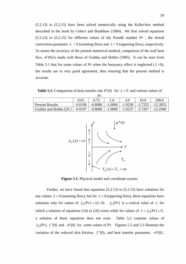
59

(5.2.13) to (5.2.15) have been solved numerically using the Keller-box method

described in the book by Cebeci and Bradshaw (1984). We first solved equations

(5.2.13) to (5.2.15) for different values of the Prandtl number Pr , the mixed

convection parameter λ > 0 (assisting flow) and λ < 0 (opposing flow), respectively.

To assess the accuracy of the present numerical method, comparison of the wall heat

flux, '(0)θ− is made with those of Grubka and Bobba (1985). It can be seen from

Table 5.1 that for some values of Pr when the buoyancy effect is neglected (λ =0),

the results are in very good agreement, thus ensuring that the present method is

accurate.

Table 5.1: Comparison of heat transfer rate )0(θ ′ for 0=λ and various values of Pr.

0.01 0.72 1.0 3.0 10.0 100.0 Present Results -0.0199 -0.8086 -1.0000 -1.9238 -3.7225 -12.3953 Grubka and Bobba [26 ] -0.0197 -0.8086 -1.0000 -1.9237 -3.7207 -12.2940 x )(* tg cxxuw =)( y ∞T axTxTw += ∞)(

Figure 5.1: Physical model and coordinate system.

Further, we have found that equations (5.2.13) to (5.2.15) have solutions for

any values 0λ > (assisting flow), but for 0λ < (opposing flow), these equations have

solutions only for values of ( ) ( 0)c Prλ λ< < . ( )c Prλ is a critical value of λ for

which a solution of equations (14) to (16) exists while for values of ( ) 0c Prλ λ< < ,

a solution of these equations does not exist. Table 5.2 contains values of

( ),c Prλ ''(0)f and '(0)θ− for some values of Pr. Figures 5.2 and 5.3 illustrate the

variation of the reduced skin friction, ''(0)f , and heat transfer parameter, '(0)θ− ,

60

with λ for some values of Pr. It can be seen from this table and figures that '(0)θ−

increases continuously with λ positive or negative, while the assisting flow ( 0)λ > ,

produces an increase in ''(0)f and an opposing flow ( 0)λ < produces a decrease in

''(0)f , respectively. We notice that increasing the value of Pr, will increase the

values of '(0)θ− that is increasing Pr enhances the heat transfer at the sheet. Thus,

fluids having a smaller Prandtl number are more sensitive to the buoyancy force than

fluids with a larger Prandtl number. These results are in agreement with those

reported by Chen (1998), see Figures 3b and 4b in his paper.

Table 5.2: Values of )0(f ′′ and )0(θ ′ for critical values of cλ (<0) and different values of Pr.

cλ )0(f ′′ - )0(θ ′ 0.70 -0.26653 -1.20032 0.69854 0.72 -0.27355 -1.20268 0.71280 1.00 -0.39356 -1.24525 0.89693 3.00 -2.01309 -1.75017 1.72057 7.00 -6.08544 -2.61278 2.67616 10.00 -9.23648 -3.11007 3.21465 50.00 -52.35663 -6.88706 7.28834 100.00 -103.75937 -10.03744 10.10021

)0(f ′′ Pr = 0.7,1,3,7,10 Pr = 0.7,1,3,7,10 λ -10 -8 -6 -4 -2 0 2 4 6 8 10 -4

-3

-2

-1

0

1

2

3

Figure 5.2: Variations of the skin friction with λ for different values of Pr.

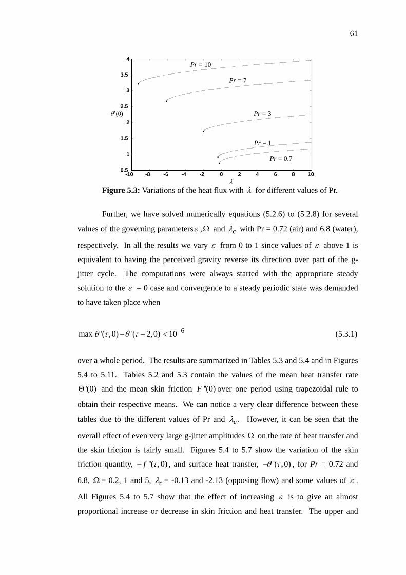
61

Pr = 10 Pr = 7

)0(θ′− Pr = 3 Pr = 1

Pr = 0.7 λ

-10 -8 -6 -4 -2 0 2 4 6 8 10 0.5

1

1.5

2

2.5

3

3.5

4

Figure 5.3: Variations of the heat flux with λ for different values of Pr.

Further, we have solved numerically equations (5.2.6) to (5.2.8) for several

values of the governing parametersε ,Ω and cλ with Pr = 0.72 (air) and 6.8 (water),

respectively. In all the results we vary ε from 0 to 1 since values of ε above 1 is

equivalent to having the perceived gravity reverse its direction over part of the g-

jitter cycle. The computations were always started with the appropriate steady

solution to the ε = 0 case and convergence to a steady periodic state was demanded

to have taken place when

6max '( ,0) '( 2,0) 10θ τ θ τ −− − < (5.3.1)

over a whole period. The results are summarized in Tables 5.3 and 5.4 and in Figures

5.4 to 5.11. Tables 5.2 and 5.3 contain the values of the mean heat transfer rate

'(0)Θ and the mean skin friction ''(0)F over one period using trapezoidal rule to

obtain their respective means. We can notice a very clear difference between these

tables due to the different values of Pr and .cλ However, it can be seen that the

overall effect of even very large g-jitter amplitudes Ω on the rate of heat transfer and

the skin friction is fairly small. Figures 5.4 to 5.7 show the variation of the skin

friction quantity, ''( ,0)f τ− , and surface heat transfer, '( ,0)θ τ− , for Pr = 0.72 and

6.8, Ω = 0.2, 1 and 5, cλ = -0.13 and -2.13 (opposing flow) and some values of ε .

All Figures 5.4 to 5.7 show that the effect of increasing ε is to give an almost

proportional increase or decrease in skin friction and heat transfer. The upper and

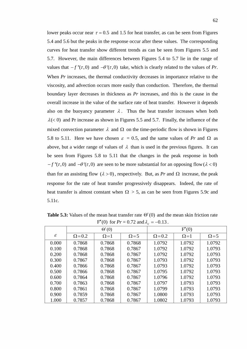
62

lower peaks occur near 0.5τ = and 1.5 for heat transfer, as can be seen from Figures

5.4 and 5.6 but the peaks in the response occur after these values. The corresponding

curves for heat transfer show different trends as can be seen from Figures 5.5 and

5.7. However, the main differences between Figures 5.4 to 5.7 lie in the range of

values that ''( ,0)f τ− and '( ,0)θ τ− take, which is clearly related to the values of Pr.

When Pr increases, the thermal conductivity decreases in importance relative to the

viscosity, and advection occurs more easily than conduction. Therefore, the thermal

boundary layer decreases in thickness as Pr increases, and this is the cause in the

overall increase in the value of the surface rate of heat transfer. However it depends

also on the buoyancy parameter λ . Thus the heat transfer increases when both

)0(<λ and Pr increase as shown in Figures 5.5 and 5.7. Finally, the influence of the

mixed convection parameter λ and Ω on the time-periodic flow is shown in Figures

5.8 to 5.11. Here we have chosen ε = 0.5, and the same values of Pr and Ω as

above, but a wider range of values of λ than is used in the previous figures. It can

be seen from Figures 5.8 to 5.11 that the changes in the peak response in both

''( ,0)f τ− and '( ,0)θ τ− are seen to be more substantial for an opposing flow ( 0)λ <

than for an assisting flow ( 0)λ > , respectively. But, as Pr and Ω increase, the peak

response for the rate of heat transfer progressively disappears. Indeed, the rate of

heat transfer is almost constant when Ω > 5, as can be seen from Figures 5.9c and

5.11c.

Table 5.3: Values of the mean heat transfer rate )0(Θ′ and the mean skin friction rate

)0(F ′′ for Pr = 0.72 and 13.0−=cλ . ε

)0(Θ′ )0(F ′′ 2.0=Ω 1=Ω 5=Ω 2.0=Ω 1=Ω 5=Ω

0.000 0.100 0.200 0.300 0.400 0.500 0.600 0.700 0.800 0.900 1.000

0.7868 0.7868 0.7868 0.7867 0.7866 0.7866 0.7864 0.7863 0.7861 0.7859 0.7857

0.7868 0.7868 0.7868 0.7868 0.7868 0.7868 0.7868 0.7868 0.7868 0.7868 0.7868

0.7868 0.7867 0.7867 0.7867 0.7867 0.7867 0.7867 0.7867 0.7867 0.7867 0.7867

1.0792 1.0792 1.0792 1.0793 1.0793 1.0795 1.0796 1.0797 1.0799 1.0800 1.0802

1.0792 1.0792 1.0792 1.0792 1.0792 1.0792 1.0792 1.0793 1.0793 1.0793 1.0793

1.0792 1.0793 1.0793 1.0793 1.0793 1.0793 1.0793 1.0793 1.0793 1.0793 1.0793

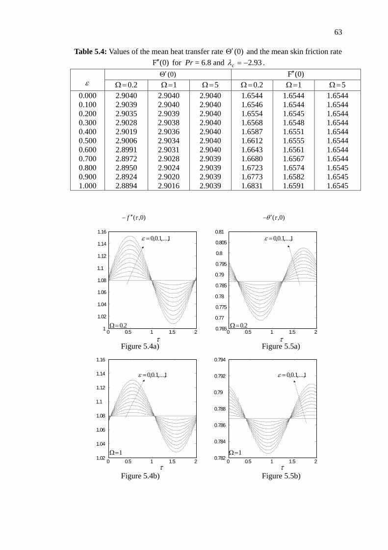
63

Table 5.4: Values of the mean heat transfer rate )0(Θ′ and the mean skin friction rate )0(F ′′ for Pr = 6.8 and 93.2−=cλ .

ε

)0(Θ′ )0(F ′′ 2.0=Ω 1=Ω 5=Ω 2.0=Ω 1=Ω 5=Ω

0.000 0.100 0.200 0.300 0.400 0.500 0.600 0.700 0.800 0.900 1.000

2.9040 2.9039 2.9035 2.9028 2.9019 2.9006 2.8991 2.8972 2.8950 2.8924 2.8894

2.9040 2.9040 2.9039 2.9038 2.9036 2.9034 2.9031 2.9028 2.9024 2.9020 2.9016

2.9040 2.9040 2.9040 2.9040 2.9040 2.9040 2.9040 2.9039 2.9039 2.9039 2.9039

1.6544 1.6546 1.6554 1.6568 1.6587 1.6612 1.6643 1.6680 1.6723 1.6773 1.6831

1.6544 1.6544 1.6545 1.6548 1.6551 1.6555 1.6561 1.6567 1.6574 1.6582 1.6591

1.6544 1.6544 1.6544 1.6544 1.6544 1.6544 1.6544 1.6544 1.6545 1.6545 1.6545

)0,(τf ′′− )0,(τθ ′− 1,...,1.0,0=ε 1,...,1.0,0=ε 2.0=Ω 2.0=Ω

τ τ0 0.5 1 1.5 21

1.02 1.04 1.06 1.08

1.1 1.12 1.14 1.16

0 0.5 1 1.5 2 0.765

0.77

0.775

0.78

0.785

0.79

0.795

0.8

0.805

0.81

Figure 5.4a) Figure 5.5a) 1,...,1.0,0=ε 1,...,1.0,0=ε 1=Ω 1=Ω τ τ

0 0.5 1 1.5 2 1.02

1.04

1.06

1.08

1.1

1.12

1.14

1.16

0 0.5 1 1.5 2 0.782

0.784

0.786

0.788

0.79

0.792

0.794

Figure 5.4b) Figure 5.5b)

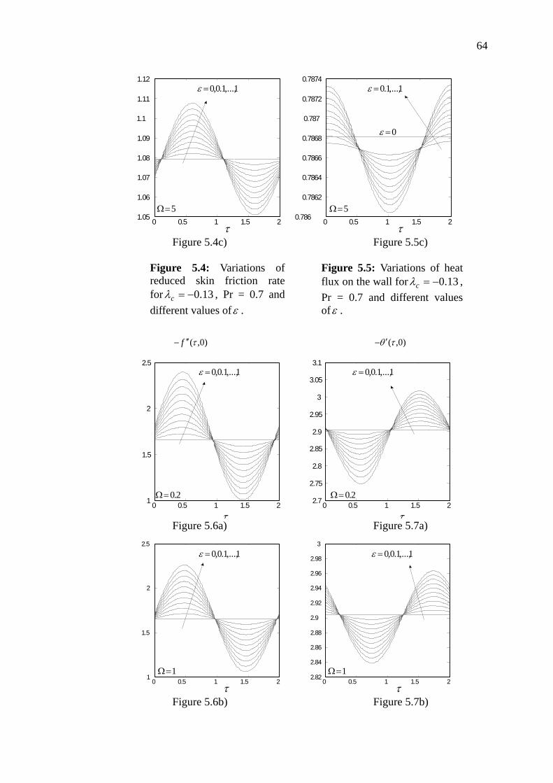
64

1,...,1.0,0=ε 1,...,1.0=ε 0=ε 5=Ω 5=Ω

τ τ 0 0.5 1 1.5 2 1.05

1.06

1.07

1.08

1.09

1.1

1.11

1.12

0 0.5 1 1.5 2 0.786

0.7862

0.7864

0.7866

0.7868

0.787

0.7872

0.7874

Figure 5.4c) Figure 5.5c)

Figure 5.4: Variations of reduced skin friction rate for 13.0−=cλ , Pr = 0.7 and different values ofε .

Figure 5.5: Variations of heat flux on the wall for 13.0−=cλ , Pr = 0.7 and different values ofε .

)0,(τf ′′− )0,(τθ ′−

1,...,1.0,0=ε 1,...,1.0,0=ε 2.0=Ω 2.0=Ω

τ τ0 0.5 1 1.5 21

1.5

2

2.5

0 0.5 1 1.5 2 2.7

2.75

2.8

2.85

2.9

2.95

3

3.05

3.1

Figure 5.6a) Figure 5.7a)

1,...,1.0,0=ε 1,...,1.0,0=ε 1=Ω 1=Ω τ τ

0 0.5 1 1.5 21

1.5

2

2.5

0 0.5 1 1.5 2 2.82

2.84

2.86

2.88

2.9

2.92

2.94

2.96

2.98

3


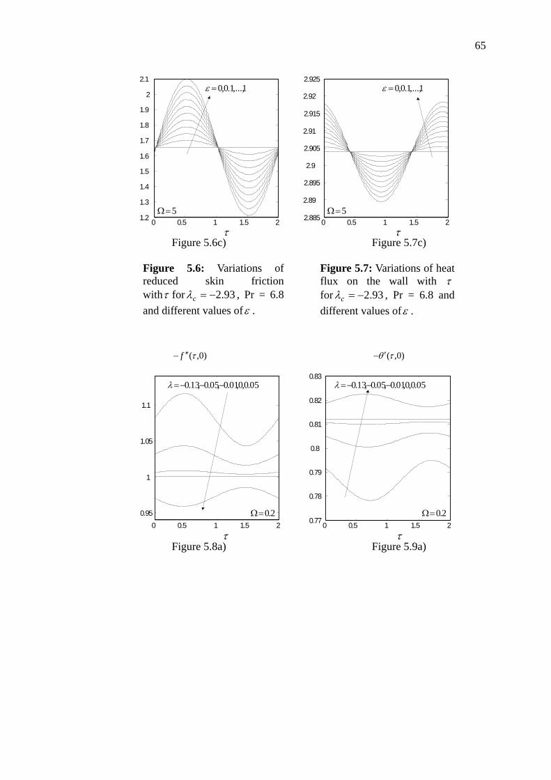
65

1,...,1.0,0=ε 1,...,1.0,0=ε 5=Ω 5=Ω

τ τ0 0.5 1 1.5 2 1.2

1.3 1.4 1.5 1.6 1.7 1.8 1.9

2 2.1

0 0.5 1 1.5 2 2.885

2.89

2.895

2.9

2.905

2.91

2.915

2.92

2.925


Figure 5.6: Variations of reduced skin friction withτ for 93.2−=cλ , Pr = 6.8 and different values ofε .

Figure 5.7: Variations of heat flux on the wall with τ for 93.2−=cλ , Pr = 6.8 and different values ofε .

)0,(τf ′′− )0,(τθ ′−

05.0,0,01.0,05.0,13.0 −−−=λ 05.0,0,01.0,05.0,13.0 −−−=λ 2.0=Ω 2.0=Ω τ τ

0 0.5 1 1.5 2 0.95

1

1.05

1.1

0 0.5 1 1.5 2 0.77

0.78

0.79

0.8

0.81

0.82

0.83


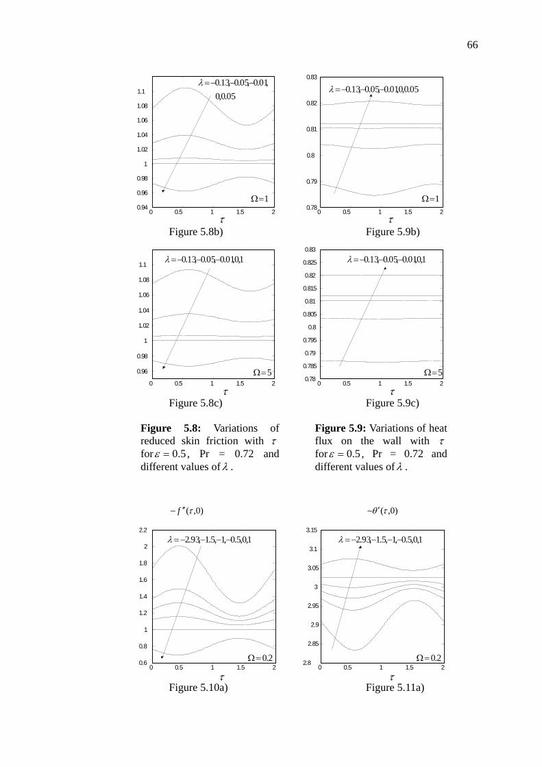
66

05.0,0

,01.0,05.0,13.0

−−−=λ 05.0,0,01.0,05.0,13.0 −−−=λ

1=Ω 1=Ω τ τ

0 0.5 1 1.5 2 0.94 0.96 0.98

1 1.02 1.04 1.06 1.08

1.1

0 0.5 1 1.5 2 0.78

0.79

0.8

0.81

0.82

0.83

Figure 5.8b) Figure 5.9b) 1,0,01.0,05.0,13.0 −−−=λ 1,0,01.0,05.0,13.0 −−−=λ 5=Ω 5=Ω τ τ

0 0.5 1 1.5 2

0.96 0.98

1 1.02 1.04 1.06 1.08

1.1

0 0.5 1 1.5 2 0.78

0.785

0.79

0.795

0.8

0.805

0.81

0.815

0.82

0.825

0.83


Figure 5.8: Variations of reduced skin friction with τ for 5.0=ε , Pr = 0.72 and different values ofλ .

Figure 5.9: Variations of heat flux on the wall with τ for 5.0=ε , Pr = 0.72 and different values ofλ .

)0,(τf ′′− )0,(τθ ′−

1,0,5.0,1,5.1,93.2 −−−−=λ 1,0,5.0,1,5.1,93.2 −−−−=λ 2.0=Ω 2.0=Ω τ τ

0 0.5 1 1.5 2 0.6 0.8

1 1.2 1.4 1.6 1.8

2 2.2

0 0.5 1 1.5 2 2.8

2.85

2.9

2.95

3

3.05

3.1

3.15


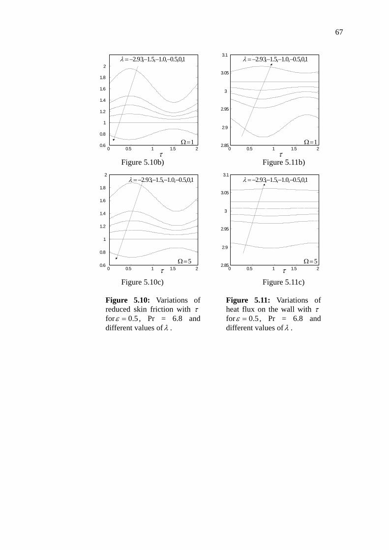
67

1,0,5.0,0.1,5.1,93.2 −−−−=λ 1,0,5.0,0.1,5.1,93.2 −−−−=λ

1=Ω 1=Ω τ τ

0 0.5 1 1.5 2 0.6 0.8

1 1.2 1.4 1.6 1.8

2

0 0.5 1 1.5 2 2.85

2.9

2.95

3

3.05

3.1


1,0,5.0,0.1,5.1,93.2 −−−−=λ 1,0,5.0,0.1,5.1,93.2 −−−−=λ 5=Ω 5=Ω τ τ 0 0.5 1 1.5 2

0.6

0.8

1

1.2

1.4

1.6

1.8

2

0 0.5 1 1.5 2 2.85

2.9

2.95

3

3.05

3.1


Figure 5.10: Variations of reduced skin friction with τ for 5.0=ε , Pr = 6.8 and different values ofλ .

Figure 5.11: Variations of heat flux on the wall with τ for 5.0=ε , Pr = 6.8 and different values ofλ .

CHAPTER VI

CONCLUSION 6.1 Summary of research

In this report we have considered two separate problems concerning the heat

transfer coefficients of a continuous stretching surface. In the first problem, we

considered the heat transfer coefficients of a continuous stretching surface subject to

uniform surface temperature, variable surface temperature and uniform heat flux. The

second problem considered is concerned with the effect of g-jitter induced free

convection adjacent to a vertical stretching sheet. Specifically, the two dimensional,

laminar and incompressible flows are considered for the first and second problems,

respectively. The problems have been solved numerically using implicit finite

difference method known as Keller-box method. Numerical results are presented

graphically and in the forms of tables.

The first problem is discussed in Chapter IV, where we have focused on the

heat transfer coefficients of a continuous stretching surface with a power law

velocity and temperature distribution 0.41 3m− ≤ ≥ and for 3 3n− ≤ ≤ . For uniform

surface temperature, ( )0n = it was found that all the temperature profile, ( )θ η

exhibit asymptotic decay for all m (see Figures 4.1, 4.2). Furthermore, the variable

surface temperature, ( )0n ≠ case is characterized by the variation of n and m. The

magnitude of n affects the direction and quantity of heat flow. For example if 3m =

and 2n = − there is no heat exchange between the surface and the ambient. On the

other hand, for 2n > − heat is transferred from continuous stretching surface to the

ambient and heat is transferred to continuous stretching surface for 3 2n− ≤ < − (see

69

Table 4.4). Finally, for uniform heat flux, ( )( )0.5 1n m= − , it was found that

increasing m, increases the quantity of heat flow to the ambient. In uniform and

variable surface temperature cases, the heat transfer coefficient, ReNu increases

with increasing m and Prandtl number (see Figures 4.3, 4.6, 4.7), however, heat

transfer coefficient, ReNu decrease with increasing m ( see Figure 4.10). In this

chapter, the plotted temperature profiles, ( )θ η decrease with increasing Prandtl

number.

In Chapter V, we have studied the problem of the effect of small but

fluctuating gravitational field, characteristic of the g-jitter, on the flow and heat

transfer adjacent to a vertical stretching sheet. The velocity and temperature of the

sheet were assumed to vary linearly with the distance x along the sheet. Effects of

the buoyancy parameter, amplitude of the g-jitter modulation, Prandtl number and

frequency of the oscillation on the flow and heat transfer characteristics have been

examined in detail. Similarity solutions have also been obtained for the case of a

steady solution, case ( 0)ε = and it was shown that for an opposing flow these

equations have solutions only for a limited range of values of the mixed convection

parameter. It can be concluded that both the skin friction and the surface heat

transfer increase as the mixed convection parameter increase for a given Pr. It is

also concluded that so long as the values of Pr and ( )c Prλ are kept constant, the

effect of increasing the values of ε is to give an almost proportional increase or

decrease in the skin friction and surface heat transfer responses. It was also shown

that for a high Prandtl number and some values of λ andΩ , the skin friction

becomes more excitable than the rate of heat transfer as can be seen from Figures 5.8

to 5.11. The gravitational modulation is more effective in investigating transition

from conductive to a convective temperature field at higher frequencies. It is hoped

that the various induced flow behaviors predicted in this work will further serve as a

well-behaved flow condition for practical microgravity processing system design and

development.

70

6.2 Suggestions for future research

There are quite a number of interesting possibilities to continue our present

research in the continuous stretching surface with power law velocity and

temperature distribution. One possibility is to consider a problem in other media and

effect such as micropolar fluid, effect of viscous dissipation and unsteady flow.

Mohammadein and Rama (2001) considered the problem for continuous stretching

surface in micropolar fluid with self similar velocity and temperature distribution

using Runge Kutta method. Therefore, our research can be continuing to use the

Keller box method to deal with the problem with power law velocity and temperature

distribution.

On the other hand, Partha et al (2005) proposed the similarity solution for a

mixed convection flow and heat transfer from an exponentially stretching surface

subject to exponential velocity and temperature distribution with effect of viscous

dissipation. The work of Partha et al (2005) can be extended by using the power law

velocity and temperature distribution. Ishak et al (2007) studied the mixed

convection on the stagnation point flow toward a vertical, continuously stretching

sheet for steady flow. We can extend Ishak et al (2007) by study their problem in

unsteady flow as well as the effect of g-jitter.

71

REFERENCES

1. Mell, W.E, Mc Grattan, K.B., Nakamura,Y., and Baum, H.R. Simulation of combustion

systems with realistic g-jitter. Sixth International Microgravity Combustion Workshop.

May 22-24, 2001. NASA Glenn Research Center, Cleveland, OH, CP-2001-210826,

2001. 333-336.

2. Yoshiaki, H., Keisuke, I., Toru, M., Satoshi, M., Shinichi, Y. and Kyoichi, K.

Numerical analysis of crystal growth of an InAs-GaAs binary semiconductor under

microgravity conditions. J. Phys. D: Appl. Phys., 2000. 33: 2508-2518.

3. Wilcox, W.R., and Regel, L.L. Microgravity effects on material processing: A Review.

Conference Proceedings of EOROMAT 2001, Rimini, Italy. July 10-14, 2001.

Associazione Italiana di Metallurgia, 1-200121 Milano, 2001. 1-9.

4. Benjapiyaporn, C., Timchenko, V., Leornadi, E. and Davis, G.D.V.Effects of space

environment on flow and concentration during directional solidification. Int. J. Fluid

Dynamics, 2000. 4: Article 3.

5. Duval, W.M.B. and Tryggvason, B.V. Effects of G-Jitter on Interfacial Dynamics of

Two Miscible Liquids: Application of MIM 37th Aerospace Sciences Meeting and

Exhibit sponsored by the American Institute of Aeronautics and Astronautics, Reno

Nevada. January 11-19, 1999. Lewis Field Cleveland, Ohio: National Aeronautics and

Space Administration, Glenn Research Center. 1999.

6. Boucher,R.L. Mechanically Induced g-jitter from Space Station Rotary Joints.

Spacebound Objective ESPACE 2000. May 14-17, 2000. The Canadian Space Agency,

Vancouver, British Colombia, 2000.

72

7. Nelson, E.S. An examination of anticipated g-jitter in Space Station and its effects on

materials processes. NASA TM 103775, 1991.

8. Monti, R., and Sovino, R. G-sensitivity of microgravity experimentation-fundamental of

disturbance response. Microgravity and Science Technology, 1998. 11. 2: 53-58.

9. Alexander J.I.D., Amirondine, S., Ouzzani, J., and Rosenberger, F. Analysis of the low

gravity tolerance of Bridgman-Stockbarger crystal growth II: Transient and periodic

acceleration: J Cryst Growth, 1991. 113(1-2): 21-38.

10. Kamotani,Y., Chao,L, A., Ostrach, S., and Zhang,H. Effect of g-jitter on free-surface

motion in a cavity. J Spacecraft and Rockets, 1995. 32, n.1: 177-183.

11. Neumann, G. Three -Dimensional Numerical simulation of buoyancy-driven convection

in vertical cylinders heated from below. J Fluid Mechanics, 1990. 214: 559-578.

12. Schneider, S.,and Straub, J. Influence of the Prandtl number on laminar natural

convection in a cylinder caused by g-jitter. Journal of Crystal Growth, 1989. 97. n.1:

235-242.

13. Pan, Bo, Shang, D-Y., Li, B.Q. and de Groh, H.C. Magnetic field effects on g-jitter

induced flow and solute transport. Int. J. Heat Mass Transfer, 2002. 45: 125-144.

14. Shu, Y., LI, B.Q., de Groh, H.C. Numerical study of g-jitter induced double diffusive

convection in microgravity. Numerical Heat Transfer B: Application, 2001. 39: 245-

265.

15. Ramos, J.I. Heat and mass transfer in annular jets: II. g-jitter. Appl. Mathematics and

Computation, 2000. 110: 165-183.

16. Li,B.Q. g-Jitter induced free convection in a transverse magnetic field. Int. of Heat and

Mass Transfer, 1996. 39: 2853-2890.

73

17. Li,B.Q. The effect of magnetic fields on low frequency oscillating natural convection.

Int. J. Engrg. Sci.,1996. 34: 1369-1383.

18. Alexander, J.I.D., Garandet J.P., Favier, J.J. and Lizee, A. g-Jitter effects on segregation

during directional solidification of tin-bismuth in the MEPHISTO furnace facility. J.

Crystal Growth, 1997. 178: 657-661.

19. Jaluria, Y. HMT The Science and Applications of Heat and Mass Transfer. Report,

Review and Computer Programs. Pergamon Press, New York. 1980.

20. Rahman M.M. and Lampinen, M.J. Numerical study of natural convection from a

vertical surface due to combined buoyancies. Numerical Heat Transfer, Part A ,1995.

28: 409-429.

21. Rees, D.A.S. and Pop, I. g-jitter induced free convection near a stagnation point. Heat

and Mass Transfer,2001. 37: 403-408.

22. Banks, W.H.H. Laminar free convection flow at a stagnation point of attachment on an

isothermal surfaces. Journal of Engineering Mathematics, 1974. 8: 45-56.

23. Bhattacharyya, S. and Gupta, A.S. MHD Flow and Heat Transfer at a General Three-

Dimensional Stagnation Point. International Journal of Non-Linear Mechanics,

1998.33: 125-134.

24. Langbein, D. Oscillatory convection in a spherical cavity due to g-jitter. ESA Mater. Sci.

under Microgravity, International Organization, 1983: 359-363.

25. Heiss, T., Schneider, S. and Straub, J. G-jitter effects on natural convection in a

cylinder: A three-dimensional numerical calculation. ESA, Proceedings of the Sixth

European Symposium on Material Sciences under Microgravity Conditions. 1987.

International Organization. 1987. 517-523.

74

26. Doi, T., Prakash, A., Azuma, H., Yoshihara, S. and Kawahara, H. Oscillatory

convection induced by g-jitter in a horizontal liquid layer. AIAA, Aerospace Sciences

Meeting and Exhibit, 33rd. Jan 9-12, 1995. Reno, NV, United States. 1995.

27. Okano, Y., Umemura, S. and Dost, S. G-jitter effect on the flow in a three-dimensional

rectangular cavity. Journal of Materials Processing and Manufacturing Science. 2001.

10(1): 3-6.

28. Gresho, P.M.,and Sani, R.L. The effects of gravity modulation on the stability of a

heated fluid layer. J. Fluid Mech,1970. 40: 783-806.

29. Biringen, S. and Peltier L.J. Computational study of 3-D Benard convection with

gravitational modulation. Phys Fluids ,1990. A 2: 279-283.

30. Biringen, S. and Danabasoglu, G. Computation of convective flow with gravity

modulation in rectangular cavities. AIAA J. Thermophys heat transfer, 1990. 4 :357-365.

31. Farooq, A., and Homsy, G.M. Streaming flows due to g-jitter induced natural

convection. J. Fluid Mech., 1994. 271 : 351-378.

32. Schlichting, H. Boundary layer theory. 7th. ed. McGraw-Hill: New York. 1979.

33. Lighthill, J. Acoustic streaming. J. Sound Vib. 1978. 61: 391-418.

34. Alexander J.I.D. Low-Gravity Experiment sensitivity to residual acceleration: A review.

Microgravity Science and Technology, 1990. III(2): 52-68.

35. Farooq, A.,and Homsy, G.M. Linear and nonlinear dynamics of a differentially heated

slot under gravity modulation. J Fluid Mech., 1996. 313 : 1-38.

36. Amin, N.The effect of g-jitter on heat transfer. Proc. R. Soc. Lond., 1988. A 419: 151-

172.

75

37. Potter, J.M. and Riley, N. Free convection from a heated sphere at large Grashof

number. J. Fluid Mech., 1980. 100: 769-783.

38. Nazar, R., Amin, N. and Pop, I. Free convection boundary layer on an isothermal sphere

in a micropolar fluid. International Communications in Heat and Mass Transfer, 2002.

29(3): 377 - 386.

39. Nazar, R., Amin, N. , Grosan, T. and Pop, I. Free convection boundary layer on a sphere

with constant heat flux in a micropolar fluid. International Communications in Heat

and Mass Transfer, 2002. 29(8): 1129 - 1138.

40. Beghein, C., Haghighata, F., Allard, F. Numerical study of double-diffusive natural

convection in a square cavity. International Journal of Heat and Mass Transfer, 1992.

35: 833-846.

41. Mahajan, R.L. and Angirasa, D. Combined heat and mass transfer by natural convection

with opposing buoyancies. Transactions of ASME Journal Heat Transfer, 1993. 115:

606-612.

42. Hussain, S., Hossain, M.A., Willson, M. Natural convection flow from a vertical

permeable flat plate with variable surface temperature and species concentration.

Engineering Computations, 2000. 17: 789-812.

43. Keller, H.B. and Cebeci,T. Accurate numerical methods in boundary-layer flows.I.

Two-dimensional laminar flows.\emph{ Proc. of the second Int. Conference on

Numerical Methods in Fluid Dynamics}. Springer, New York, 1971. 92-100.

44. Paterson, W.R and Hayhurst, A.N. Mass or heat transfer from a sphere to flowing fluid.

Chemical Engineering Science, 2000. 55: 1925-1927.

45. Elperin, T. and Fominykh, A. Effect of solute concentrate level on the rate of coupled

mass and heat transfer during solid sphere dissolution in a uniform fluid flow. Chemical

Engineering Science, 2001. 56: 3065-3074.

76

46. Sharidan, S., Amin, N. and Pop, I. g-Jitter fully developed heat and mass transfer by

mixed convection flow in a vertical channel. International Communications in Heat

and Mass Transfer, 2005. 32: 657 - 665.

47. Jue, T.C. and Ramaswamy, B. Numerical analysis of thermosolutal flows in a cavity

with gravity modulation effects. Heat and Mass Transfer, 2002. 38(7-8): 665-672.

48. Slouti, A., Takhar, H.S. and Nath, G. Unsteady free convection flow in the stagnation-

point region of a three-dimensional body. International Journal Heat and Mass

Transfer, 1998. 41: 3397-3408.

49. Lok, Y.Y., Amin, N. and Pop, I. Unsteady boundary layer flow of a micropolar fluid

near the rear stagnation point of a plane surface. Int. J. Thermal Sci., 2003. 42: 995-

1001.

50. Rosenhead, D. Laminar Boundary Layers. Oxford University Press, London. 1962.

51. Meksyen, D. New Methods in Laminar Boundary Layer Theory. Pergamon, New York.

1961.

52. Wang, C.Y. Axisymmetric Stagnation Point Flow on a Cylinder. Q. Appl. Math,

1974.32: 207-213.

53. Sano, S and Wakitani, S. Unsteady Free Convection Near a Forward Stagnation Point at

Small Prandtl Number. Journal of the Physical Society of Japan, 1984. 53: 1277-1283.

54. Amin N, and Riley, N. Mixed Convection at a Stagnation Point. Quarterly Journal

Mechanics and Applied Mathematics, 1995. 48: 111-121.

55. Amin N, and Riley N. Free Convection at an Axisymmetric Stagnation Point. Journal of

Fluid Mechanics, 1996. 314: 105-112.

77

56. Seshadri, R., Sreeshylan, N. and Nath, G. Unsteady Mixed Convection Flow in the

Stagnation Region of a Heated Vertical Plate Due to Impulsively Motion. International

Journal of Heat and Mass Transfer, 2002. 45: 1345-1352.

57. Nazar, R., Amin, N. and Pop, I. Unsteady Mixed Convection Near the Forward

Stagnation Point of a Two-Dimensional Symmetric Body. International

Communications in Heat and Mass Transfer, 2003. 30: 673-682.

58. Rees, D.A.S. and Pop, I. The effect of g-jitter on a free convection near a stagnation

point in a porous medium. Int. of Heat and Mass Transfer, 2001. 44: 877-883.

59. Rees, D.A.S.and Pop, I.The effect of g-jitter on vertical free convection boundary-layer

in a porous medium. Int. comm. Heat Mass Transfer, 2000. 27 : 415-424.

60. Rees, D.A.S. and Pop, I. The effect of large-amplitude g-jitter vertical free convection

boundary layer flow in porous media. International Journal of Heat and Mass Transfer,

2003. 46: 1097-1102

61. Unsworth, K. and Chiam, T.C. A numerical solution of the two-dimensional boundary

layer equations for micropolar fluids. J. Appl. Math. Mech. (ZAMM), 1981. 61: 463-466.

62. Gorla, R.S.R., Takhar, H.S., Slaouti, A. and Pop, I. and Kumari, M. Free convection in

power-law fluids near a three-dimensional stagnation point. International Journal Heat

and Fluid Flow, 1995. 16: 62-68.

63. Peddieson, J. and McNitt, R.P. Boundary layer theory for a micropolar fluid. Recent

Adv. in Engng. Sci., 1970. 5: 405-476.

64. Guram, G.S. and Smith, C. Stagnation flows of micropolar fluids with strong and weak

interactions. Comp. Math.with Applics., 1980. 6: 213-233.

65. Lok, Y.Y., Phang, P., Amin, N. and Pop, I. Unsteady flow of a micropolar fluid near the

forward and rear stagnation points. Int. J. Engng. Sci., 2003. 41: 173-186.

78

66. Kumari, M. and Nath, G. Unsteady incompressible boundary layer flow of a micropolar

fluid at a stagnation point. Int. J. Engng. Sci., 1984. 22: 755-768.

67. Lok, Y.Y., Amin, N. and Pop, I. Steady two-dimensional asymmetric stagnation point

flow of a micropolar fluid. J. Appl. Math. Mech. (ZAMM), 2003. 83: 594-602.

68. Howarth, L. The boundary layer in three-dimensional flow. Part II. The flow near a

stagnation point. Philos. Mag.,1951. 42: 1433-1440.

69. Poots, G. Laminar free convection on the lower stagnation point on an isothermal

curved surface. International Journal of Heat and Mass Transfer, 1964. 7: 863-873.

70. Banks, W.H.H. Three-dimensional free convection flow near a two-dimensional surface.

Journal of Engineering Mathematics, 1972. 6: 109-115.

71. Ingham, D.B., Merkin, J.H. and Pop, I. Unsteady free convection of a stagnation point

of attachment on an isothermal surface. International Journal Mathematics and

Mathematical Science, 1984. 7: 599-614.

72. Keller, H. B. and Cebeci, T. (1972). Accurate Numerical Methods for Boundary Layer

Flows, II: Two-Dimensional Turbulent Flows, AIAA Journal. 10: 1193-1199.

73. Cebeci, T. and Bradshaw, P. (1977). Momentum Transfer in Boundary Layers.

Washington: Hemisphere.

74. Ali, M. E. (1994). Heat transfer characteristics of a continuous stretching surface

W¨arme Stoff¨ubertragung. 29: 227–34.

75. Cebeci, T. and Bradshaw, P. (1988). Physical and Computational Aspects of

ConvectiveHeat Transfer. New York: Springer.

76. Chen, C.H (1998). Laminar mixed convection adjacent to vertical, continuously

stretching sheets. Heat and Mass Transfer. 33: 471–476.

79

77. Bejan, A. (1984). Convection Heat Transfer. New York: John Wiley.

78. Ghoshdastidar, P.S. (2004). Heat Transfer. Oxford University Press.

79. Ali, M E. (1995) On thermal boundary layer on a power-law stretched surface with

suction or injection Int. J. Heat Mass Flow. 16: 280–90.

80. Crane, L.J.: Flow past a stretching plane. J. Appl. Math. Phys. (ZAMP), vol. 21, p. 645

(1970).

81. Magyari, E., Keller, B.: Heat and mass transfer in the boundary layers on an

exponentially stretching continuous surface. J. Phys. D: Appl. Phys., vol. 32, p. 577

(1999).

82. Magyari, E., Keller, B.: Exact solutions for self-similar boundary-layer flows induced

by permeable stretching surfaces. Eur. J. Mech. B-Fluids, vol. 19, p. 109 (2000).

83. Nazar, R., Amin, N., Pop, I.: Unsteady boundary layer flow due to a stretching surface in a

rotating fluid. Mechanics Res. Comm., vol. 31, p. 121 (2004).

84. Daskalakis, J.E.: Free convection effects in the boundary layer along a vertically stretching

flat surface. Canad. J. Phys., vol. 70, p. 1253 (1993).

85. Ali, M.E., Al-Yousef, F.: Laminar mixed convection from a continuously moving vertical

surface with suction or injection. Heat Mass Transfer, vol. 33, p. 301(1998).

86. Chen, C.-H.: Laminar mixed convection adjacent to vertical, continuously stretching

sheets. Heat Mass Transfer, vol. 33, p. 471 (1998).

87. Chen, C.-H.: Mixed convection cooling of heated continuously stretching surface. Heat

Mass Transfer, vol. 36, p. 79 (2000).

88. Lin, C.-R., Chen, C.-K.: Exact solution of heat transfer from a stretching surface with

80

variable heat flux. Heat Mass Transfer, vol. 33, p. 477 (1998).

89. Chamkha, Ali J.: Hydromagnetic three-dimensional free convection on a vertical stretching

surface with heat generation or absorption. Int. J. Heat Fluid Flow, vol. 20, p. 84 (1999).

90. Kumari, M., Slaouti, A., Takhar, H.S., Nakamura, S., Nath, G.: Unsteady free convection

flow over a continuous moving vertical surface. Acta Mechanica, vol. 116, p. 75 (1996).

91. Antar, B.N., Nuotio-Antar, V.S.: Fundamentals of Low Gravity Fluid Dynamics and

Heat Transfer. CRC Press, Boca Raton, FL, 1993.

92. Hirata, K., Sasaki, T., Tanigawa, H.: Vibrational effects on convection in a square cavity

at zero gravity. J. Fluid Mech., vol. 445, p. 327 (2001).

93. Alexander, J.I.D.: Low gravity experiments sensitivity to residual acceleration: A

review. Microgravity Sci. Techol., vol. III 2, p. 52(1990).

94. Nelson, E.: An examination of anticipated g-jitter on space station and its effects on

material processing. NASA Tech. Mem., No. 103775 (1991).

95. Amin, N.: The effect of g-jitter on heat transfer. Proc. R. Soc. London, vol. A 419, p. 151

(1988).

96. Farooq, A., Homsy, G.M.: Streaming flows due to g-jitter induced natural convection. J.

Fluid Mech., vol. 271, p. 351 (1994).

97. Li, B.Q.: g-Jitter induced free convection in a transverse magnetic field. Int. J. Heat


98. Li, B.Q.: The effect of magnetic fields on low frequency oscillating natural convection.

Int. J. Engng. Sci., vol. 34, p. 1369 (1996).

99. Pan, B., Li, B.Q.: Effect of magnetic fields on oscillatory mixed convection. Int. J. Heat

81


100. Rees, D.A.S., Pop, I.: The effect of g-jitter on vertical free convection boundary layer in

a porous medium. Int. Comm. Heat Mass Transfer, vol. 27, p. 415 (2000).

101. Rees, D.A.S., Pop, I.: The effect of g-jitter on free convection near a stagnation point in

a porous medium. Int. J. Heat Mass Transfer, vol. 44, p. 877 (2001).

102. Rees, D.A.S., Pop, I.: g-Jitter induced free convection near a stagnation point. Heat


103. Chamkha, Ali J.: Effects of heat generation on g-jitter induced natural convection flow

in a channel with isothermal or isoflux walls. Heat Mass Transfer, vol. 39, p. 553

(2003).

104. Cebeci, T., Bradshaw, P.: Physical and Computational Aspects of Convective Heat

Transfer. Springer, New York, 1984.

105. Grubka, L.J., Bobba, K.M.: Heat transfer characteristics of a continuous, stretching

surface with variable temperature. J. Heat Transfer, vol. 107, p. 248 (1985).

LAPORAN AKHIR PROJEK PENYELIDIKAN FRGS VOT: … · LAPORAN AKHIR PROJEK PENYELIDIKAN FRGS VOT:...

Documents

Transcript of LAPORAN AKHIR PROJEK PENYELIDIKAN FRGS VOT: … · LAPORAN AKHIR PROJEK PENYELIDIKAN FRGS VOT:...