Longitudinal Dispersion of Pollutants in Natural Streams...

Pertanika J. Sci. & Technol. 1(2): 225-238 (1993)ISSN: 0128-7680

© Universiti Pertanian Malaysia Press

Longitudinal Dispersion of Pollutants in NaturalStreams - The Aggregated Dead-Zone Approach

Mohd. Nasir HassanDepartment of Environmental Sciences

Universiti Pertanian Malaysia43400 Serdang, Selangor Darl Ehsan, Malaysia

Received 6 January 1992

ABSTRAK

Model Agrigat Zon-Tetap (ADZ) memberi gambaran ringkas mengenai dinamikpergerakan dan penyerakan bahan cemar di dalam sungai yang tidak mempunyaisifat pasang surut. Ianya merupakan satu pilihan terhadap model AlirlintangPenyerakan yang lebih rumit. Artikel ini memeparkan keputusan yang di dapatihasH dari penggunaan model ADZ untuk sistem sungai. Keputusan menunjukkanbentuk urnurn fungsi perkaitan di antara parameter orde kedua model ADZdengan luahan sungai. Suhubungan dengan itu juga, analisis hidrologi secaralazim telah menghasilkan maklumat penting mengenai ciri-ciri hidraulik sungaidan memberi ruang dari segi perbandingan cara ini dengan parameter ADZ.

ABSTRACT

The Aggregated Dead-Zone (ADZ) model provides a simple dynamic description of pollutant transportation and dispersion in a non-tidal river system andis an alternative to the well-known but more complicated advection-dispersionmodel. This paper presents the results obtained from the application of themodel in a river system. The study shows the general form of functionalrelationships between the second order ADZ model parameters and streamdischarge. In addition, more conventional hydrological analysis has yieldedvaluable information about the hydraulic characteristics of the reaches and hasallowed for useful comparisons between these and the ADZ model parameters.

Keywords: pollutants, dispersion, transportation, advectioIHtispersion model, Aggregated Dead-Zone model, effective volwne, ADZ residence time

INTRODUCTION

Studies on dispersion processes in rivers are widely used by hydrodynamicists,hydrologists and environmental scientists involved in the study of waterpollution problems. The time of travel of a pollutant in a river or estuary,the rate at which the pollutant spreads out, the decrease in peak concentration and the resulting concentration patterns of pollutant are theimportant variables that must be properly understood. Serious pollutionmay result if the capacity of a stream to transport and disperse a contaminant is overestimated. Underestimation on the other hand may result invaluable resources not being optimally utilised, resulting in unnecessaryexpenditure on treatment facilities. It has been emphasised that virtuallyno water quality management study which is aimed at achieving optimum

Mohd. Nasir Hassan

usage of a river or estuarine system can bypass the need for a reliablemeans of predicting the dispersion characteristics of the water body(Sooky 1969).

There have been many studies on longitudinal dispersion of pollutantsin rivers and natural streams. The best-known study, usually quoted intexts on the subject, is the Fickian theory. It was developed for flow inpipes by Taylor (1954) and extended to channels by Elder (1959) and fornatural streams by Fischer (1966). Their research involved a mathematicalrepresentation in the form of a single dimensional, partial differentialequation, usually known as the one-dimensional Fickian Diffusion model.In this model, dispersion is quantified by the effective longitudinal dispersion coefficient, usually termed the "Dispersion Coefficient". Much efforthas been extended in order to measure and/or estimate the dispersioncoefficient (Harris 1963; Fischer 1968; Bansal 1971; Liu 1977; Fischer et al.1979; Chatwin & Allen 1985). However, the apparent popularity of theFickian-type model is not fully justified by its performance in practicalapplications. When used for the characterisation of dispersion in naturalstreams, it has not always been successful (e.g. Day 1975; Sabol & Nordin1978; Bencala & Walters 1983; Legrand-Marc & Laudelout 1985). Inparticular, the temporal profiles observed at fixed locations on the riverappear often to have sharper rises times and longer tails than thosepredicted by the Fickian-type model; while in non-uniform streams, thelongitudinal dispersion coefficients, as described by Taylor (1954) andElder (1959), vary considerably and consistently from those associated withthe normal distribution. Subsequently, various studies have investigatedalternative models which are better able to represent the observed "nonFickian" behaviour in channels and natural streams. Amongst the mostsuccessful of these alternative models and the most recent is the aggregated dead-zone model (ADZ) developed by Young (1982), Beer & Young(1983), Young (1983) and Young & Wallis (1986). The model argues that,while Fickian-type dispersion is probably taking place to some extent, mostof the dispersion observed in natural streams arises because of the deadzone effects caused by irregularities in river beds and banks. In otherwords, it is assumed that the cumulative effects of the dead-zones oftendominate the observed dispersion and they can be amalgamated in theirtotal effect to yield an "Aggregated Dead-Zone (ADZ)" whose "residencetime" then defines the dispersion properties associated with the stretch ofriver being studied.

In this paper, we describe the results obtained from application of theADZ model in a river system. It presents the physical interpretation of themodel and also explores the relationships between various ADZ parameters and physical variables such as stream discharge and the volume ofwater in the reach.

226 Pertanika J. Sci. & Techno!. Vo!. 1 No.2, 1993

Longitudinal Dispersion of Pollutants in Natural Streams

The Aggregated Dead-Zone ModelThe simplest way of developing the ADZ model is to consider a typicaldead-zone with volume Vi in a steady flow field with a rate Q. Then, underthe assumption of complete mixing and a conservative solute, the relationship between the input concentration u(t) and the output concentrationx(t) of the solute in the dead-zone is obtained from a dynamic massbalance, as follows:

d[Vjx(t)] = Q u(t) Q x(t)

dt (1)

rate of change mass in per mass out perin the dead-zone unit mass unit mass

If for simplicity we assume that both Vi and Q are constant, then theequation for a conservative solute can be written,

dx(t)

dt

Q x(t)

V1

+Q u(t)

V1

(2)

Equation (2) describes the dispersion processes of a single dead-zonewhich may occur anywhere in the stream. Between any two points, therecan be a number of such dead-zones with different volumes, all contributing to the total dispersive properties of the stream as a series ofinterconnected processes. Thus, in the aggregated dead-zone model, it isassumed that the aggregated effect of all these processes can be describedby a small number of "effective" dead-zones. In the simplest case, only onesuch aggregated dead-zone is necessary for the reach. If its volume is V

e,

the effective volume, then the ADZ model for the reach would be:

dx(t) Q x(t)

Ve

+Q u(t)

Ve

(3)

where x(t) and u(t) now represent the overall input and output soluteconcentrations associated with the ADZ for the whole reach.

The ADZ provides the basic mechanism for dispersion in a given reachof a river. However, advective effects also playa major role in the transportof solute down a river (Young 1984). In the Fickian Diffusion model theseare introduced by the advective term and controlled by the stream velocity.In the ADZ model a pure time delay is ino::oduced into the input term toallow for the pure translational effect of the river flow. Equation (3) thenbecomes:

Pertanika J. Sci. & Techno!. Vo!. 1 No.2, 1993 227

Mohd. Nasir Hassan

d x(t)- Cl'x(t) + a u(t-r) (4)

dtwhere r is the pure time delay and a = Q/V

e•

Equation (4) represents a basic equation for a single aggregated deadzone. It is a first order differential-delay equation. Using Laplace Transforms (Schwarzenbach & Gill 1984), the unit impulse response of Equation (4) is in the form of a simple, time-delayed, exponential decayfunction as follows:

x(t) (5)

where the time constant T = II CI' =VJQ is called the ADZ residence time.Equation (4) describes the transportation and dispersion properties of

a given reach. In order to describe a complete river system it is necessaryto combine an appropriate number of such elements in a pattern definedby the physical nature of the river under study. To determine the numberof ADZ elements required to represent the specified length of river in amulti-reach model it is convenient to consider the alternative discretetime, sampled data version of the ADZ model. This not only allows for anobjective evaluation but also helps in the implementation of the modeland the construction of a stochastic framework around the model, i.e. aframework which has considerable advantages for use of the model inapplications such as planning, management, forecasting and control. Also,data obtained from pollution monitoring are often in sampled form andas such, the discrete-time model provides its most natural characterisation.

There are many ways of deriving a discrete-time version of the ADZmodel (i.e. equation 4), but the simplest and most straightforward isobtained by assuming that the input u(t) is constant over the discretisationinterval T,. With this assumption about u( t), the discrete-time version ofthe equation takes the following form,

(6)

where the subscript k indicates the value of the associated variable at thekth sampling instant and 8, the nearest integral of TITs' is the transportation time delay in sampling intervals. In the simplest case, the parameters 'a' and 'b' in Equation (6) are related to the continuous-time modelparameters by the following equation,

T V/Q = -T/ln(-a);be s 1 + a (7)

228 Pertanika J. Sci. & Techno!. Vol. 1 No.2, 1993


It should be noted however, that both these equations and thedefinition of the discrete time delay in Equation (6) introduce approximations which may necessitate some alteration in the basic model form toallow for additional parameters and a modification of the relationships in(7) .

Equation (6) can be transformed into operator form by the introduction of the backward shift operator z, i.e.

In this manner, it is straightforward to develop the following discrete-timetransfer function form of equation (6).

1 + a z·t

A general, multi-order form of this model can be written as follows,

(8)

(9)

where n and m are integers whose values will be determined by the natureof the transportation and dispersion in the river systems (Young 1984). Ingeneral, n represents the number of first order ADZ elements required todescribe the observed dispersion properties of the reach, while m willdepend on factors such as the presence of non-integral pure time delay orthe presence of additional parallel dead zones.

A general approach to modelling water quality in rivers is described byBeck (Orlob 1983). He discussed all aspects of model calibration andverification within a useful unified framework. More specific time seriesmodels such as equation (10), and their application to general hydrological problems, are discussed by Young (1983, 1984) and Young & Wallis(1986). For the research described in this paper, computer programs existfor processing data obtained from tracer studies carried out on the riverin order to statistically "identify" the k=model order (n and m) and theassociated time delay, and to then "estimate" the parameters ai' i = 1 ton, and b, j = 0 to m, as in equation (9).

The particular computer program employed in this study is the microCAPTAIN program, which uses recursive Instrumental variable (IV) methods of identification and estimation (Young 1984). This process of identification and estimation can be considered as the statistical equivalent ofthe better-known, but more closely defined, "calibration" procedures used


Mohd. Nasir Hassan

in the construction of non-conventional water quality simulation modelssuch as QUAL II (Orlob 1983). They have the advantage of allowingmodel builders to objectively evaluate the model structure which is mostappropriate to the characterisation of their field data. In other words, thetime-series helps to obviate the construction of a model which may have areach structure which is more complicated than necessary.

In order to apply statistical identification and estimation procedures toany dynamic model, it is necessary to consider the model in stochasticterms. The major advantages associated with such a stochastic formulationare that (a) it allows the power of statistical methodology to be applied tomodel calibration, and (b) it provides a means of quantifying the uncertainty associated with both the model parameter estimates and any forecasts made with the help of the model. As regards (a), the microCAPTAINprogram provides two main statistics for assessing model adequacy (Younget at. 1980). First, the ability of the model to explain the data is evaluatedby a Coefficient of Determination (~2) which represents a normalisedmeasure of model fit, with a value of unity indicating a perfect explanationof the time-series data and zero specifying modelling errors of the sameorder of magnitude as the output data. Second, the precision of the modelparameter estimates is indicated by an Error Variance Norm (EVN) , whichrepresents an overall measure of the error variance associated with themodel parameter estimates and tends to increase sharply in value whenthe selected model order (the number of ADZ elements in the multi-orderADZ model) is greater than that justified by the data.

The modelling procedure used in microCAPTAIN is based on therepeated evaluation of these two statistics for different order models (i.e.for different values of n, m and 8): the best identified model is thenselected as the model which simultaneously provides a good explanationof data, as indicated by a low relative value of R/, and well definedparameter estimates, as indicated by a high relative value for the EVN. Inparticular, as the number of model parameters is increased so ~2 tendstowards a "plateau" with very little improvement markedly when the modelhas too many parameters, illustrating the large increase in uncertainty thataccompanies over-parameterisation. Because it may increase by severalorders of magnitude following the onset of over-parameterisation, theEVN is normally represented by its natural logarithm, In EVN.

EXPERIMENTAL TECHNIQUES AND DATA PROCESSING

Experimental SitesThe ADZ model study involved dilution gauging methods in selectedreaches in Crimple Beck (Beven 1976). It is a catchment area nearHarrogate, Yorkshire, comprising small, rocky, steep and rough channels.Flow in selected streams is characterised by slow pool segments, past rime



and rapid segments, waterfalls, and other irregularities in the channel bedcreating rapid changes in flow depth and width.

In the experiment, common salt in solution was injected as a singleinput (slug) at a selected upstream point in the reach. The concentrationof salt was subsequently measured at the downstream stations using aportable electrical conductivity meter. The conductivity measurementswere then converted to an equivalent concentration of salt by a calibrateddilution of a sample of the input solution with distilled water.

The distance between the point of injection of salt and the samplingpoint downstream was 30 metres and because of the relative roughness ofthe stream this offered complete mixing of the tracer. Studies conductedby Beven (1976) showed that the Darcy-Weisbach roughness coefficient (j)was seen to decrease with increasing discharge but at low flows the valuesare very high. The highest fvalue recorded was 12 and this is equivalentto a Manning n of > 1. Eighteen experiments were carried out withdischarges varying between 4 and 190 litres/second.

Data ProcessingIn order to describe the transportation and dispersion of pollutant usingthe ADZ model, two types of observed data were required: the upstream(input) and the downstream (output) data. The measured downstreamdata were taken from the salt concentration-time data gathered in thedilution-gauging experiments. The output data was compiled at a sampling interval of 15 to 30 seconds.

In the experiments, the upstream (input) data are not the realobserved data since Beven (1976) only documented the downstream(output) observations. However, as the common salt solution was injectedas a pulse, it is possible to synthesise the input data in the form of an"impulsive" response. This was carried out in the following manner:

(1) At t = 0, the input concentration is U gil. We will see that the U valueis, to some extent, arbitrary. However, it was assumed for the moment thatit is larger than the maximum observed output data.(2) When t> 0, then the input concentration is zero.

In addition to ADZ model parameter estimation, the data analysis alsoincludes more conventional hydrological calculations. These include themean travel time t which is obtained as the real time difference betweenthe centroid locations of the input data and the observed output concentration-time profiles. Knowing the value of t and the discharge Q, otherhydraulic parameters related to the ADZ model can be calculated. Theyare the reach volume (V), ADZ residence time (T), ADZ effective volume(V) and the V/V ratio.

Pertanika J. Sci. & Techno!. Vo!. I No.2, 1993 231

Mohd. Nasir Hassan

RESULTS AND DISCUSSION

The results of the study are presented and discussed in two parts:estimation of the ADZ model i.e. the identification and estimation of theADZ model order; and the physical description of the ADZ.

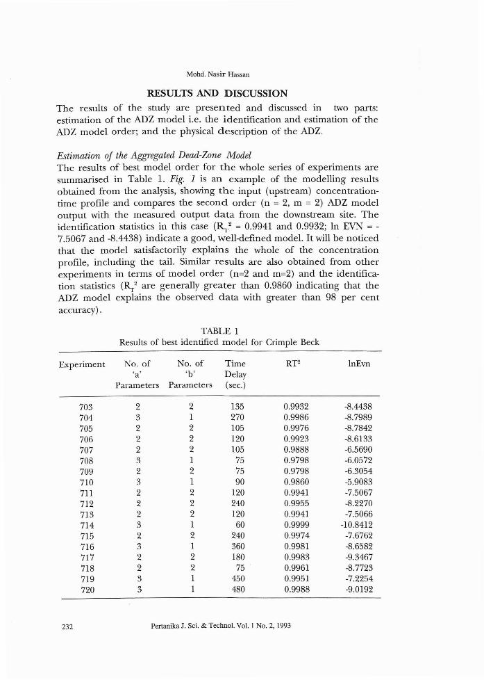
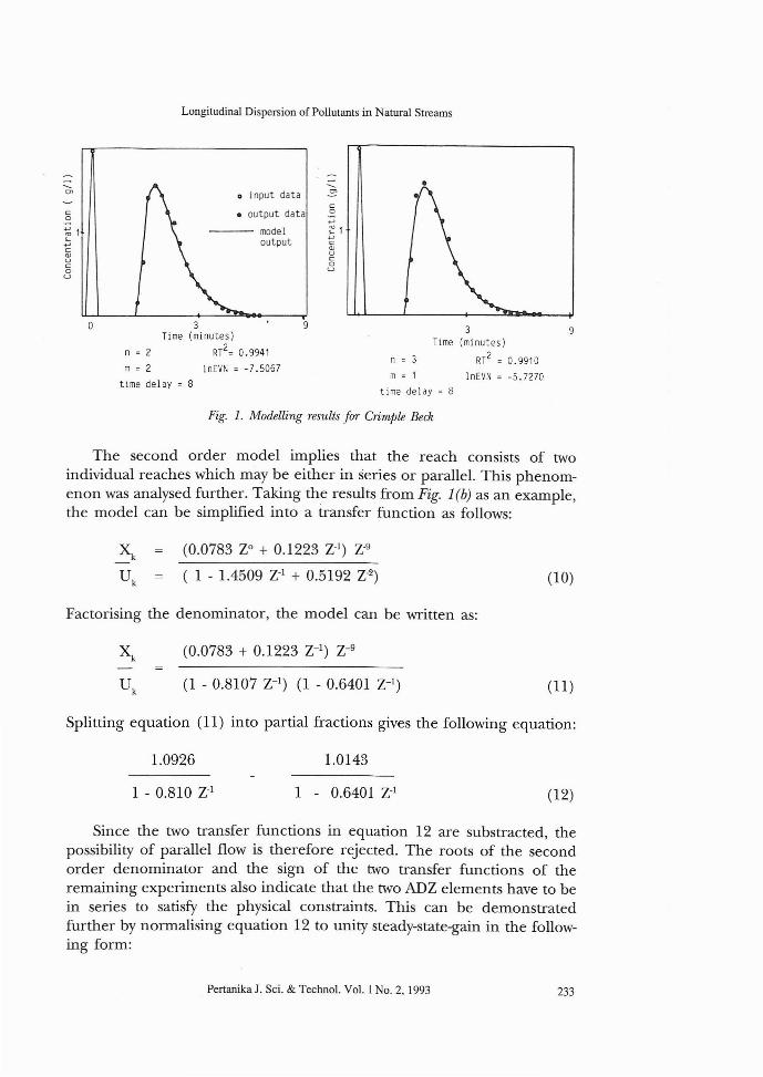
Estimation of the Aggregated Dead-Zone ModelThe results of best model order for the whole series of experiments aresummarised in Table 1. Fig. 1 is an example of the modelling resultsobtained from the analysis, showing the input (upstream) concentrationtime profile and compares the second order (n = 2, m = 2) ADZ modeloutput with the measured output data from the downstream site. Theidentification statistics in this case (~2 = 0.9941 and 0.9932; In EVN = 7.5067 and -8.4438) indicate a good, well-defined model. It will be noticedthat the model satisfactorily explains the whole of the concentrationprofile, including the tail. Similar results are also obtained from otherexperiments in terms of model order (n=2 and m=2) and the identification statistics (~2 are generally greater than 0.9860 indicating that theADZ model explains the observed data with greater than 98 per centaccuracy).

TABLE 1Results of best identified model for Crimple Beck

Experiment No. of No. of Time RT2 InEvn'a' 'b' Delay

Parameters Parameters (sec.)

703 2 2 135 0.9932 -8.4438704 3 1 270 0.9986 -8.7989705 2 2 105 0.9976 -8.7842706 2 2 120 0.9923 -8.6133707 2 2 105 0.9888 -6.5690708 3 1 75 0.9798 -6.0572709 2 2 75 0.9798 -6.3054710 3 1 90 0.9860 -5.9083711 2 2 120 0.9941 -7.5067712 2 2 240 0.9955 -8.2270713 2 2 120 0.9941 -7.5066714 3 1 60 0.9999 -10.8412715 2 2 240 0.9974 -7.6762716 3 1 360 0.9981 -8.6582717 2 2 180 0.9983 -9.3467718 2 2 75 . 0.9961 -8.7723719 3 1 450 0.9951 -7.2254720 3 1 480 0.9988 -9.0192

232 Pertanika J. Sci. & Technol. Vol. 1 No.2, 1993


3Time (minutes)

RT2 = 0.9910

InEVN = -5.7270

n = 3

m = 1

time delay = 8

c:o...~ 1...c:QJUc:ou

o input data

• output data

--- modeloutput

3 9Time (minutes)

n = 2 RT2= 0.9941

m = 2 InEVN = -7.5067

time delay = 8

o

c:o

~1s......c:QJuc:ou

Fig. 1. Modelling results for Crimple Beck

The second order model implies that the reach consists of twoindividual reaches which may be either in series or parallel. This phenomenon was analysed further. Taking the results from Fig. 1(b) as an example,the model can be simplified into a transfer function as follows:

(0.0783 ZO + 0.1223 Z-I) Z-9

( 1 - 1.4509 Z-I + 0.5192 Z-2) (10)

Factorising the denominator, the model can be written as:

~ (0.0783 + 0.1223 Z-I) Z-9

(1 - 0.8107 Z-I) (1 - 0.6401 Z-I) (11)

Splitting equation (11) into partial fractions gives the following equation:

1.0926 1.0143

1 - 0.810 Z-I 1 - 0.6401 Z-I (12)

Since the two transfer functions in equation 12 are substracted, thepossibility of parallel flow is therefore rejected. The roots of the secondorder denominator and the sign of the two transfer functions of theremaining experiments also indicate that the two ADZ elements have to bein series to satisfy the physical constraints. This can be demonstratedfurther by normalising equation 12 to unity steady-state-gain in the following form:


1x

Mohd. Nasir Hassan

0.0783 (l + 1.56 z-r) z-g2.946 (1 - 0.81 z-r) (1 - 0.64 Z-I)

0.0266 (l + 1.156 Z-I) z-g(1 - 0.81 Z-I) (l - 0.64 Z-I) (13)

where 1/2.946 is the normalisation allowed by the arbitrary choice of u;the steady-state-gain now is equal to unity (SSG=I). The transfer functioncan be rewritten as:

Advection (A) ADZ 1 (B)

0.19

1- 0.81 Z-I

ADZ 2 (C)

0.36

1 - 0.64 Z-I

where block A represents the advective effects (pure-time delay of 9sampling periods) and the value 0.39 + 0.61 Z-l is to allow for theadditional "non-integral" time delay which gives rise to the requirementsfor the 2 "b" parameters. Blocks Band C represent 2 unequal ADZelements in series.

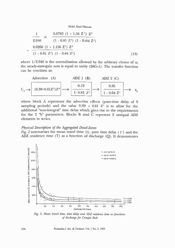
Physical Description of the Aggregated Dead-ZonesFig. 2 summarises the mean travel time (t), pure time delay ( r) and theADZ residence time (T) as a function of discharge (Q). It demonstrates

-;;;-"0

8 1200

!E" 1000§

"g~'in 800E!N0-<:

:S 600~a;"0

".§400

13".§~ 200~c.."::i

T.l01+3076/0

T' 66.9+1578/0

T' 33.9+1498/0

20 40 60 80 100 120 140 160 180 200

Discharge (0) (Vsecs)

234

Fig. 2. Mean travel time, time delay and ADZ residence time as functionsof discharge for Crimple Beck

Pertanika J. Sci. & Technol. Vol. 1 No.2, 1993


that these parameters exhibit a relatively smooth functional relationshipwith discharge, with the parameters decreasing with Q as might beexpected from physical considerations. The curves however, level out as Qincreases. Similar relationships have been found by Beven (1976), Beltaos(1982) and Young & Wallis (1986).

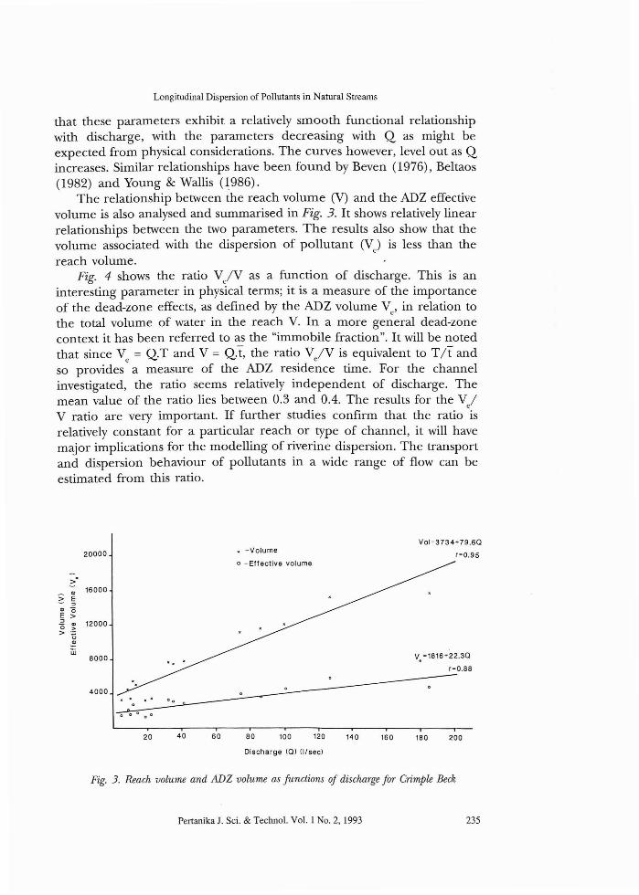
The relationship between the reach volume (V) and the ADZ effectivevolume is also analysed and summarised in Fig. 3. It shows relatively linearrelationships between the two parameters. The results also show that thevolume associated with the dispersion of pollutant (V) is less than thereach volume.

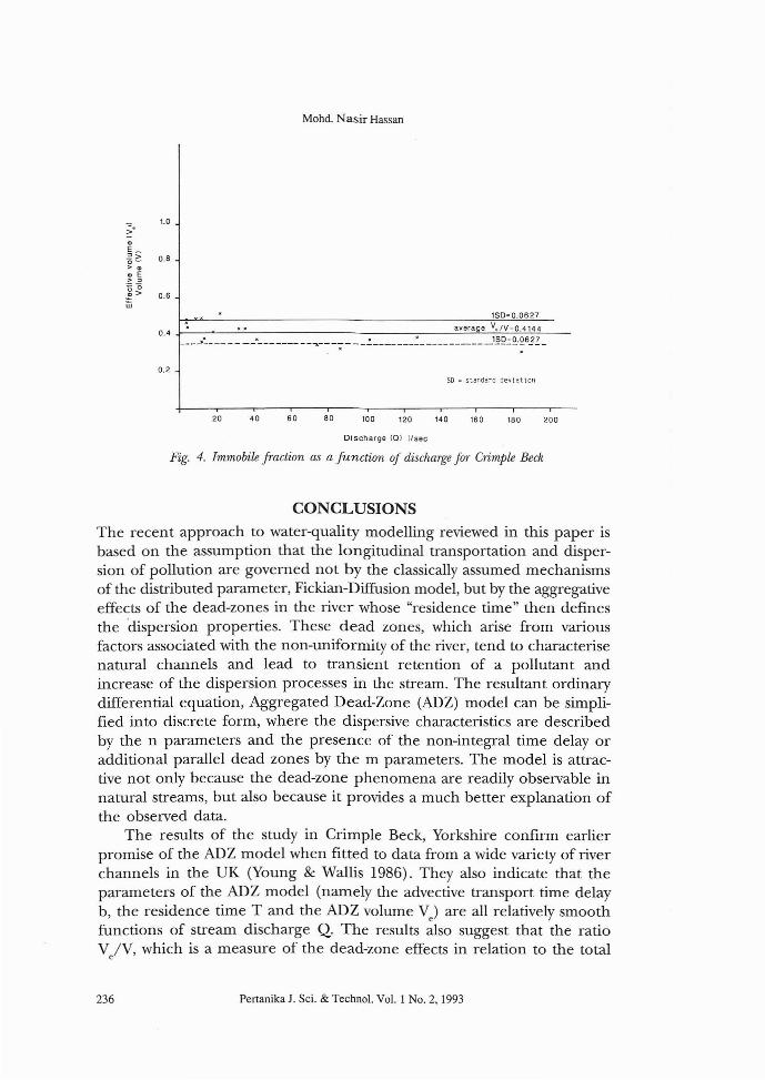
Fig. 4 shows the ratio V/V as a function of discharge. This is aninteresting parameter in physical terms; it is a measure of the importanceof the dead-zone effects, as defined by the ADZ volume V , in relation to

e

the total volume of water in the reach V. In a more general dead-zonecontext it has been referred to as the "immobile fraction". It will be notedthat since V

e= Q.T and V = Q.t, the ratio V/V is equivalent to T/t and

so provides a measure of the ADZ residence time. For the channelinvestigated, the ratio seems relatively independent of discharge. Themean value of the ratio lies between 0.3 and 0.4. The results for the V /

e

V ratio are very important. If further studies confirm that the ratio isrelatively constant for a particular reach or type of channel, it will havemajor implications for the modelling of riverine dispersion. The transportand dispersion behaviour of pollutants in a wide range of flow can beestimated from this ratio.

20000

>'

'"16000

~ E

"'" (;E >" '" 12000(; >>

"~Ui8000 .'.

.4000

>I -Volume

o -Effective volume

Vol-3734+79.6Q

r-0.95

V. =1816+22.3Q

r=0.88

20 40 60 80 100 120 140 160 180 200

Discharge (Q) II/sec)

Fig. 3. Reach volume and ADZ volume as functions of discharge for Crimple Beck


Mohd. Nasir Hassan

1.0:;.

0.8

0.6

tSO-0.0627

0.4 ..I--_~----=..:...... ----:;__.::.:av""er..::Ja""e-:V:::,./~V-"O'0"?.4:,,,14c:c4____ -,"- ' ~_--_;- __~ .: ,§Q.:2..2.6.?Z_

0.2so ,. standard deviation

20 40 60 80 100 '20 140 160

Discharge (Q) I/sec

180 200

Fig. 4. Immobile fraction as a function of discharge fO"r Crimple Beck

CONCLUSIONS

The recent approach to water-quality modelling reviewed in this paper isbased on the assumption that the longitudinal transportation and dispersion of pollution are governed not by the classically assumed mechanismsof the distributed parameter, Fickian-Diffusion model, but by the aggregativeeffects of the dead-zones in the river whose "residence time" then definesthe dispersion properties. These dead zones, which arise from variousfactors associated with the non-uniformity of the river, tend to characterisenatural channels and lead to transient retention of a pollutant andincrease of the dispersion processes in the stream. The resultant ordinarydifferential equation, Aggregated Dead-Zone (ADZ) model can be simplified into discrete form, where the dispersive characteristics are describedby the n parameters and the presence of the non-integral time delay oradditional parallel dead zones by the m parameters. The model is attractive not only because the dead-zone phenomena are readily observable innatural streams, but also because it provides a much better explanation ofthe observed data.

The results of the study in Crimple Beck, Yorkshire confirm earlierpromise of the ADZ model when fitted to data from a wide variety of riverchannels in the UK (Young & Wallis 1986). They also indicate that theparameters of the ADZ model (namely the advective transport time delayb, the residence time T and the ADZ volume V.) are all relatively smoothfunctions of stream discharge Q. The results also suggest that the ratioV IV, which is a measure of the dead-zone effects in relation to the total

e



water volume in the reach at any time, appears to be relatively independent of discharge. This opens up the possibility of calibrating the reach inADZ terms from the results of only a small number of dilution-gauging ordye- tracer experiments.

REFERENCESBANSAL, M.K. 1971. Dispersion in natural streams. J. Hydraul. Div. Proc. ASCE 97: 1967

1986.

BEER, T. and P.C. YOUNG. 1983. Longitudinal dispersion in natural streams. J. Environ.Eng. ASCE. 109:1049-1067.

BELTAOS, S. 1982. Dispersion in tumbling flow. J. Hydraul. Div. Proc. ASCE 108: 591-611.

BENCALA, K.E. and R.A. WALTERS. 1983. Simulation of solute transport in a mountainpool-and-riffle stream: a transient storage model. Water Resour. Res. 19: 718-724.

BEVEN, K.F. 1976. Obtaining bulk channel routing parameters by dilution gaugingmethods. Working paper No. 146, Department of Geography, University of Leeds.

CHATWIN, P.C. and C.M. ALLEN. 1985. Mathematical models of dispersion in rivers andestuaries. Ann. Rev. Fluid Mechanics 17:119-149.

DAY, T.J. 1975. Longitudinal dispersion in natural channels. Water Resour. Res. 11: 909918.

ELDER, J.W. 1959. The dispersion of marked fluid in turbulent shear flow. J. FluidMechanics 5: 544-560.

FISCHER, H.B. 1966. A note on the one-dimensional dispersion model. Air and WaterPollution Int. J. 10:443-453.

FISCHER, H.B. 1968. Dispersion predictions in natural streams. J. Sanit. Eng. Proc. 94: 927943.

FISCHER, RB., EJ. LIST, J. IMBERGER and N.H. BROOKS. 1979. Mixing in Inland and CoastalWaters. New York: Academic Press. 483pp.

HARRIS, E.K. 1963. A new statistical approach to the one- dimensional diffusion model.Air and Water Pollution Int. J. 7: 799-812.

LEGRAND-MARc, C. and H. UUDELOUT. 1985. Longitudinal dispersion in a forest stream.J. Hydrol. 78: 317-324.

LIU, H. 1977. Predicting dispersion coefficients of streams. J. Environ. Eng. Div. Proc.ASCE. 103: 56-69.

ORLOB, GT. (ed). 1983. Mathematical Modelling of Water Quality: Streams, Lakes andReservoirs. New York: J. Wiley.

SABOL, G.V. and C.F. NORDIN. 1978. Dispersion in rivers as related to storage zone. J.Hydraulic Division. Proc. ASCE. 104: 695-708.

SCHWARZENBACH, J. and K.F. GILL. 1984. System Modelling and Control. Victoria: EdwardArnold. pp. 322.


Mohd. Nasir Hassan

SOOKY, A. 1969. Longitudinal dispersion in open channel. J Hydraulic Division. Proc.ASCE. 95: 1327-1345.

TAYLOR, G.!. 1954. Dispersion of soluble matter in solvent flowing through a tube. Proc.R Sac. Landon. Series A. 219: 186-203.

YOUNG, P.C. 1975. Recursive approach to time-series analysis. Bull. Inst. Matks. Applic. 10:209-224.

YOUNG, P.C. 1982. The validity and credibility of models for badly defined systems. InUncertainty and Forecasting of Water Qyality, ed. M.B. Beck and G.V. Stratan. Berlin:Springer Verlag.

YOUNG, P.C. 1983. System methods in the evaluation of environmental pollutionproblems. In Pollution - Causes, Effects and ControL ed. R.M. Harrison. Royal Soc.Chemistry.

YOUNG, P.c. 1984. Recursive Estimation and Time Series Analysis - An Introduction. Berlin:Springer Verlag.

YOUNG, P.c., AJ.JAKEMAN and R. Me MURTRIE. 1980. An instrumental variable method formodel order identification. Automatica 16: 281-294.

YOUNG, P.C. and S.G. WALLIS. 1986. The aggregated dead zone model for dispersion inrivers. In Froc. Int. Conf. Water Qyality Modelling in Inland Natural Environment.Bournemouth. BHRA: p. 421-437.


Longitudinal Dispersion of Pollutants in Natural Streams...

Documents

Transcript of Longitudinal Dispersion of Pollutants in Natural Streams...