66:2 (2014) 85–89 | www.jurnalteknologi.utm.my | eISSN 2180–3722 |

Full paper Jurnal

Teknologi

Numerical Analysis of Hydrodynamic Propeller Performance of LNG Carrier in Open Water M. Nakisaa, A. Maimunb*, Yasser M. Ahmeda, Jaswara, A. Priyantoa, F. Behrouzia

aFaculty of Mechanical Engineering, Universiti Teknologi Malaysia, 81310 UTM Johor Bahru, Johor, Malaysia bMarine Technology Centre, Universiti Teknologi Malaysia, 81310 UTM Johor Bahru, Johor, Malaysia

*Corresponding author: Adi@fkm.utm.my

Article history

Received :1 July 2013 Received in revised form :

15 July 2013

Accepted :11 December 2013

Graphical abstract

Hydrodynamic propeller performance

In open water

Abstract

Marine propeller blade geometries, especially LNG carriers, are very complicated and determining the hydrodynamic performance of these propellers using experimental work is very expensive, time

consuming and has many difficulties in calibration of marine laboratory facilities. This paper presents the

assessment on the effect of turbulent model and mesh density on propeller hydrodynamic parameters. Besides that, this paper focuses on the LNG carrier Tanaga class propeller hydrodynamic performance

coefficients such as Kt, Kq and η, with respect to the different advance coefficient (j). Finally, the results

from numerical simulation that were calculated based on RANS (Reynolds Averaged Navier Stocks) equations, were compared with existing experimental results, followed by analysis and discussion

sections. As a result the maximum hydrodynamic propeller efficiency occurred when j=0.84.

Keywords: Numerical simulation; LNG carrier; hydrodynamic parameters; propeller; RANS equation

© 2014 Penerbit UTM Press. All rights reserved.

1.0 INTRODUCTION

Nowadays, viscid and in-viscid flows with CFD (Computational

Fluid Dynamics) are widely used for design aims and the

experimental tests to be conducted for the last step of research

work. Considering to in maritime applications, numerical methods

can be performed to estimate the flow pattern around ship hulls,

rudders, propellers and appendages.

In case of the visualisation of flow pattern around merchant

ship’s propellers, computational fluid dynamics based on Lifting-

Surface theory for first step is commonly used [1 and 3]. The

viscid RANS (Reynolds Average Navier Stocks) equation

solution was used later comes to function after [2].

Reynolds Average Navier Stocks is introduced for the

application of numerical technics in fluid mechanics and

improvement on computer performances. [4, 6, 7 and 8].

Modelling, geometry, computational domains, boundary

conditions, topology, meshing method and mesh size and

turbulent method have significant effects on a fruitful numerical

analysis and accuracy of simulation. Meshing strategy is divided

in two divisions. Hybrid unstructured a mesh means that the

tetrahedral elements for flow fluid fields, while structured mesh

means that the hexahedral mesh is totally used for meshing on the

solid surfaces. In contrast, the results of simulations with

structured mesh elements usually have more accuracy than

tetrahedral mesh elements results.

Unstructured mesh elements production is almost automatic while

hexahedral mesh elements generation is not automatic and should

be generated manually. On the other hand, for flow field meshing,

sometimes, the geometry is not compatible to use the hexahedral

mesh elements, so unstructured mesh elements have better results

and convergence of solution is nice. Therefore, we used the

hybrid unstructured mesh elements for rotational domain, in

which we utilized the stationary and rotational domain for full

scale propeller simulation for propeller with five blades.

CFD simulation data were verified with existing tests results.

This study focuses on hydrodynamic propeller performance and

characteristics in open water condition. The hydrodynamic values

such as thrust (Kt) and torque (Kq) coefficients and the other

selected values were measured in this numerical research work.

2.0 PROPELLER MODEL

The propeller model with full scale principles was simulated in

this numerical work using finite volume method. The diameter

(D) of considered propeller was 7.7 m and the diameter of hub

(Dhub) was 0.17D, plus the rotation of the propeller was made

right handed to make the thrust. Pitch ratio design (P/D) was 0.94

and blade ration (EAR) was 0.88.

The propeller drawing is depicted in Figure 1 and the Table 1

shows the geometric characteristics.

86 A. Maimun et al. / Jurnal Teknologi (Sciences & Engineering) 66:2 (2014), 85–89

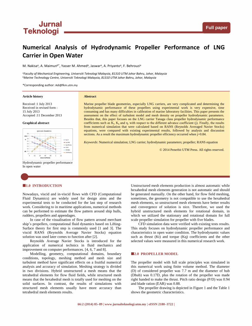
Figure 1 Front view of propeller

The centreline of the propeller was allocated on the centre

point and reference of the Cartesian coordination. The x-direction

was associated with centreline of the propeller, y-direction was

arranged with upward of the propeller and z-direction followed

the right handed Cartesian coordination system that showed to

port side, as shown in Figure 1.

Table 1 Propeller geometric characteristics

Parameters Dimension

Z 5

D 7.7 m

Dhob 1.28 m

Br 0.17

P/D 0.94

Ae/A0 0.88

R 15 Deg.

3.0 BOUNDARY CONDITION

ANSYS-Fluent 13 was applied to numerical prediction of the

hydrodynamic propeller characteristics which solved the RANS

equation by finite volume method. Figure 2 and Table 2 show the

scheme and dimensions of computational domain to simulate the

propeller in open water, respectively.

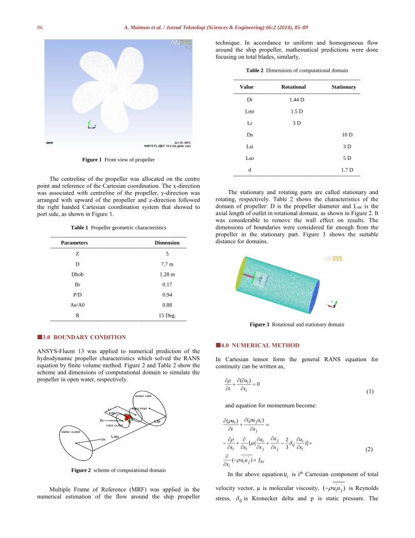
Figure 2 scheme of computational domain

Multiple Frame of Reference (MRF) was applied in the

numerical estimation of the flow around the ship propeller

technique. In accordance to uniform and homogeneous flow

around the ship propeller, mathematical predictions were done

focusing on total blades, similarly.

Table 2 Dimensions of computational domain

Value Rotational Stationary

Dr

1.44 D

Lmr

1.5 D

Lr

3 D

Ds

10 D

Lsi

3 D

Lso

5 D

d 1.7 D

The stationary and rotating parts are called stationary and

rotating, respectively. Table 2 shows the characteristics of the

domain of propeller: D is the propeller diameter and Lmr is the

axial length of outlet in rotational domain, as shown in Figure 2. It

was considerable to remove the wall effect on results. The

dimensions of boundaries were considered far enough from the

propeller in the stationary part. Figure 3 shows the suitable

distance for domains.

Figure 3 Rotational and stationary domain

4.0 NUMERICAL METHOD

In Cartesian tensor form the general RANS equation for

continuity can be written as,

0)(

i

i

x

u

t

(1)

and equation for momentum become:

j

iji

x

uu

t

u )()(

bijii

i

iij

j

j

j

i

ii

fuux

x

u

x

u

x

u

xx

)(

)]3

2([

''

(2)

In the above equationiu is ith Cartesian component of total

velocity vector, µ is molecular viscosity, )( ''jiuu is Reynolds

stress, ij is Kronecker delta and p is static pressure. The

87 A. Maimun et al. / Jurnal Teknologi (Sciences & Engineering) 66:2 (2014), 85–89

Reynolds stress should be demonstrated to near the governing

equations by suitable turbulent model. For solution the RANS

equation and turbulence velocity time scale, it is used by

Boussinesq’s eddy-viscosity supposition and two transport

equations. The body force is expressed by fbi.

For determination the 3D viscous incompressible flow

around the ship’s hull is used the ANSYS-CFX14.0 code. The

parallel version of CFX concurrently calculates the flow

formulations using numerous cores of computers. The shear stress

transport (SST) turbulence model had been used in this study,

because it gave the best results in comparison with other

turbulence models. The equations are shown as follows:

Equation of k :

(3)

Equation of :

SYGxx

ux jj

iit

)()()( (4)

Where kG and G express the generation of turbulence

kinetic energy due to mean velocity gradients and . k and

express the active diffusivity of k and . kY and Y represent the

dissipation of k and due to turbulence. D expresses the cross-

diffusion term, kS and S are user-defined source terms Further

detail is available in [9].

5.0 RESULT AND DISCUSSION

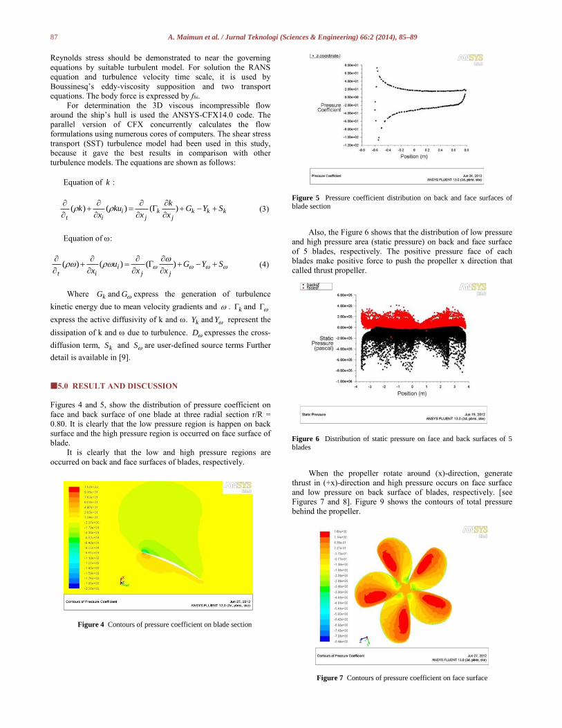
Figures 4 and 5, show the distribution of pressure coefficient on

face and back surface of one blade at three radial section r/R =

0.80. It is clearly that the low pressure region is happen on back

surface and the high pressure region is occurred on face surface of

blade.

It is clearly that the low and high pressure regions are

occurred on back and face surfaces of blades, respectively.

Figure 4 Contours of pressure coefficient on blade section

Figure 5 Pressure coefficient distribution on back and face surfaces of

blade section

Also, the Figure 6 shows that the distribution of low pressure

and high pressure area (static pressure) on back and face surface

of 5 blades, respectively. The positive pressure face of each

blades make positive force to push the propeller x direction that

called thrust propeller.

Figure 6 Distribution of static pressure on face and back surfaces of 5

blades

When the propeller rotate around (x)-direction, generate

thrust in (+x)-direction and high pressure occurs on face surface

and low pressure on back surface of blades, respectively. [see

Figures 7 and 8]. Figure 9 shows the contours of total pressure

behind the propeller.

Figure 7 Contours of pressure coefficient on face surface

kkkj

kj

iit

SYGx

k

xku

xk

)()()(

88 A. Maimun et al. / Jurnal Teknologi (Sciences & Engineering) 66:2 (2014), 85–89

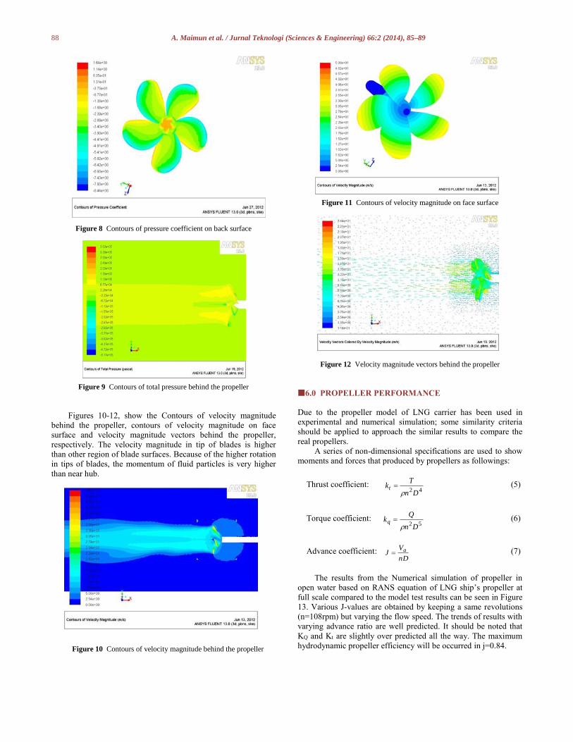
Figure 8 Contours of pressure coefficient on back surface

Figure 9 Contours of total pressure behind the propeller

Figures 10-12, show the Contours of velocity magnitude

behind the propeller, contours of velocity magnitude on face

surface and velocity magnitude vectors behind the propeller,

respectively. The velocity magnitude in tip of blades is higher

than other region of blade surfaces. Because of the higher rotation

in tips of blades, the momentum of fluid particles is very higher

than near hub.

Figure 10 Contours of velocity magnitude behind the propeller

Figure 11 Contours of velocity magnitude on face surface

Figure 12 Velocity magnitude vectors behind the propeller

6.0 PROPELLER PERFORMANCE

Due to the propeller model of LNG carrier has been used in

experimental and numerical simulation; some similarity criteria

should be applied to approach the similar results to compare the

real propellers.

A series of non-dimensional specifications are used to show

moments and forces that produced by propellers as followings:

Thrust coefficient: 42Dn

Tkt

(5)

Torque coefficient: 52Dn

Qkq

(6)

Advance coefficient: nD

VJ a (7)

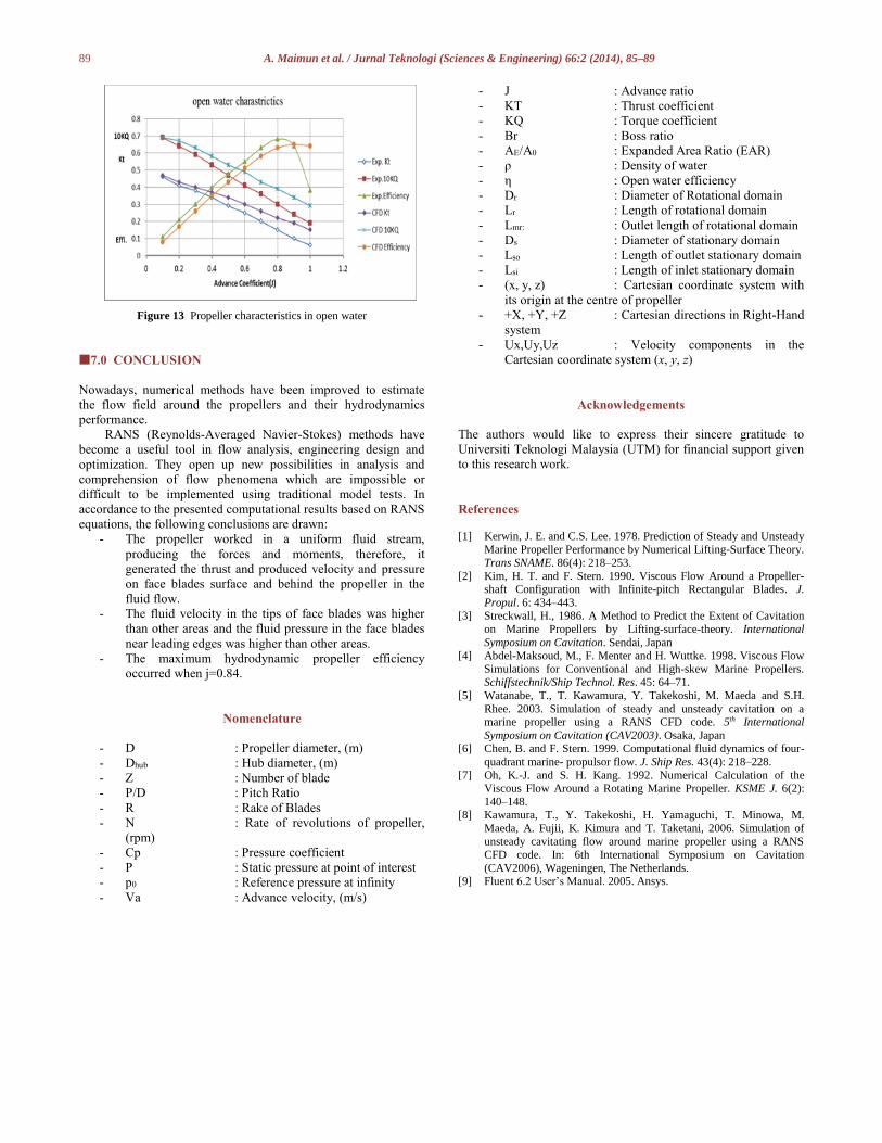
The results from the Numerical simulation of propeller in

open water based on RANS equation of LNG ship’s propeller at

full scale compared to the model test results can be seen in Figure

13. Various J-values are obtained by keeping a same revolutions

(n=108rpm) but varying the flow speed. The trends of results with

varying advance ratio are well predicted. It should be noted that

KQ and Kt are slightly over predicted all the way. The maximum

hydrodynamic propeller efficiency will be occurred in j=0.84.

89 A. Maimun et al. / Jurnal Teknologi (Sciences & Engineering) 66:2 (2014), 85–89

Figure 13 Propeller characteristics in open water

7.0 CONCLUSION

Nowadays, numerical methods have been improved to estimate

the flow field around the propellers and their hydrodynamics

performance.

RANS (Reynolds-Averaged Navier-Stokes) methods have

become a useful tool in flow analysis, engineering design and

optimization. They open up new possibilities in analysis and

comprehension of flow phenomena which are impossible or

difficult to be implemented using traditional model tests. In

accordance to the presented computational results based on RANS

equations, the following conclusions are drawn:

- The propeller worked in a uniform fluid stream,

producing the forces and moments, therefore, it

generated the thrust and produced velocity and pressure

on face blades surface and behind the propeller in the

fluid flow.

- The fluid velocity in the tips of face blades was higher

than other areas and the fluid pressure in the face blades

near leading edges was higher than other areas.

- The maximum hydrodynamic propeller efficiency

occurred when j=0.84.

Nomenclature

- D : Propeller diameter, (m)

- Dhub : Hub diameter, (m)

- Z : Number of blade

- P/D : Pitch Ratio

- R : Rake of Blades

- N : Rate of revolutions of propeller,

(rpm)

- Cp : Pressure coefficient

- P : Static pressure at point of interest

- p0 : Reference pressure at infinity

- Va : Advance velocity, (m/s)

- J : Advance ratio

- KT : Thrust coefficient

- KQ : Torque coefficient

- Br : Boss ratio

- AE/A0 : Expanded Area Ratio (EAR)

- ρ : Density of water

- η : Open water efficiency

- Dr : Diameter of Rotational domain

- Lr : Length of rotational domain

- Lmr: : Outlet length of rotational domain

- Ds : Diameter of stationary domain

- Lso : Length of outlet stationary domain

- Lsi : Length of inlet stationary domain

- (x, y, z) : Cartesian coordinate system with

its origin at the centre of propeller

- +X, +Y, +Z : Cartesian directions in Right-Hand

system

- Ux,Uy,Uz : Velocity components in the

Cartesian coordinate system (x, y, z)

Acknowledgements

The authors would like to express their sincere gratitude to

Universiti Teknologi Malaysia (UTM) for financial support given

to this research work.

References

[1] Kerwin, J. E. and C.S. Lee. 1978. Prediction of Steady and Unsteady

Marine Propeller Performance by Numerical Lifting-Surface Theory.

Trans SNAME. 86(4): 218–253.

[2] Kim, H. T. and F. Stern. 1990. Viscous Flow Around a Propeller-shaft Configuration with Infinite-pitch Rectangular Blades. J.

Propul. 6: 434–443. [3] Streckwall, H., 1986. A Method to Predict the Extent of Cavitation

on Marine Propellers by Lifting-surface-theory. International

Symposium on Cavitation. Sendai, Japan [4] Abdel-Maksoud, M., F. Menter and H. Wuttke. 1998. Viscous Flow

Simulations for Conventional and High-skew Marine Propellers. Schiffstechnik/Ship Technol. Res. 45: 64–71.

[5] Watanabe, T., T. Kawamura, Y. Takekoshi, M. Maeda and S.H.

Rhee. 2003. Simulation of steady and unsteady cavitation on a marine propeller using a RANS CFD code. 5th International

Symposium on Cavitation (CAV2003). Osaka, Japan [6] Chen, B. and F. Stern. 1999. Computational fluid dynamics of four-

quadrant marine- propulsor flow. J. Ship Res. 43(4): 218–228.

[7] Oh, K.-J. and S. H. Kang. 1992. Numerical Calculation of the Viscous Flow Around a Rotating Marine Propeller. KSME J. 6(2):

140–148. [8] Kawamura, T., Y. Takekoshi, H. Yamaguchi, T. Minowa, M.

Maeda, A. Fujii, K. Kimura and T. Taketani, 2006. Simulation of

unsteady cavitating flow around marine propeller using a RANS CFD code. In: 6th International Symposium on Cavitation

(CAV2006), Wageningen, The Netherlands. [9] Fluent 6.2 User’s Manual. 2005. Ansys.