Review of Parameter Estimation Techniques for Time-Varying … · 2016-06-28 · Moreover, the...
6
Review of Parameter Estimation Techniques for Time-Varying Autoregressive Models of Biomedical Signals A. R. Najeeb, M. J. E. Salami, T. Gunawan, and A. M. Aibinu Department of Electrical and Computer Engineering, International Islamic University of Malaysia, Kuala Lumpur, Malaysia Email: {athaur, momoh, teddy}@iium.edu.my, [email protected] Abstract—Biomedical signals are non-stationary and a research topic of practical interest as the signal has time varying statistics. The problem of time varying is usually circumvented by assuming local stationary over a short time interval, where stationary techniques are applied. However, features extracted from these methods are not always suitable and methods for non-stationary process are needed. Time varying signals are more accurately represented by time frequency methods and received most attention recently. Among the time frequency methods, parametric modeling such as TVAR has been promising over non- parametric methods with improved resolutions and able to trace strong non-stationary signal. Despite the success of TVAR in various applications it has drawbacks. This paper presents an extensive review on TVAR modelling techniques. Different approaches for TVAR modeling is presented and outlined. Principles, advantages, disadvantages of those techniques are presented concisely. And finally a new direction has been suggested briefly. Index Terms—autoregressive spectral analysis, biomedical signal processing, model order determination, non- stationary signal analysis time varying coefficients, genetic algorithm, artificial neural network I. INTRODUCTION A common routine for dealing with non-stationary signal is to partition into several segments (window) of known length; after which traditional methods of nom- parametric methods or parametric method such as Fast Fourier Transform (FFT) or Autoregressive (AR) is applied [1]. The signal is assumed to be stationary within this short-duration window; however, this method may not work well if averaging of Power Spectral Density (PSD) from different segments fails to capture the dynamics of the data [2]. Furthermore, each segment is assumed to be independent but for many signals, this is not the case as each segment is statistically depends on the next. While some data turn out to be too short, leading to that the estimates become unreliable due to few data points and cannot partitioned into several segments. This has led to a growing interest in non-stationary signal processing including Time-Frequency Representation Manuscript received February 10, 2015; revised July 13, 2015. (TFR) techniques which able to capture changing dynamics of both deterministic and random signal. TFR also works well with short data. Available TFR methods are categorized into non-parametric methods and parametric methods as shown in Fig. 1. Figure 1. Classification of non-stationary signal analysis The most extensively exploited non-parametric method includes Short Term Fourier Transform (STFT), Smoothed Pseudo Wigner-Ville (SPWV), Wavelet Transforms, Gabor Transform (GT), Hilbert Transform (HT), Continuous Mortlet Wavelet Transform (CMWT), Wigner-Viler (WVD) and their enhanced derivations. These methods are computational efficient and do not make any assumptions about the process except for its stationarity, which makes them as methodology of choice particularly in situations where long data need to be analyzed. A good summary of properties, mathematical model and application of these techniques can be found in [2]-[5]. Despite their success, there are some drawbacks of these methods, for example, the window effects, the low time-frequency resolution in STFT and the cross-term interference in WD. STFT is essentially composed of piece-wise FFT, which assumes that the signal is locally stationary in each segment The segment size is so critical to performance as there exist a trade-off between time resolution and frequency resolution in accordance with uncertainty principle [6]. Choosing a short segment size causes poor frequency resolution while a long segment size compromises the assumption of stationary data [7]. International Journal of Signal Processing Systems Vol. 4, No. 3, June 2016 ©2016 Int. J. Sig. Process. Syst. 220 doi: 10.18178/ijsps.4.3.220-225
Transcript of Review of Parameter Estimation Techniques for Time-Varying … · 2016-06-28 · Moreover, the...
Review of Parameter Estimation Techniques for
Time-Varying Autoregressive Models of
Biomedical Signals
A. R. Najeeb, M. J. E. Salami, T. Gunawan, and A. M. Aibinu Department of Electrical and Computer Engineering, International Islamic University of Malaysia, Kuala Lumpur,
Malaysia
Email: {athaur, momoh, teddy}@iium.edu.my, [email protected]
Abstract—Biomedical signals are non-stationary and a
research topic of practical interest as the signal has time
varying statistics. The problem of time varying is usually
circumvented by assuming local stationary over a short time
interval, where stationary techniques are applied. However,
features extracted from these methods are not always
suitable and methods for non-stationary process are needed.
Time varying signals are more accurately represented by
time frequency methods and received most attention
recently. Among the time frequency methods, parametric
modeling such as TVAR has been promising over non-
parametric methods with improved resolutions and able to
trace strong non-stationary signal. Despite the success of
TVAR in various applications it has drawbacks. This paper
presents an extensive review on TVAR modelling techniques.
Different approaches for TVAR modeling is presented and
outlined. Principles, advantages, disadvantages of those
techniques are presented concisely. And finally a new
direction has been suggested briefly.
Index Terms—autoregressive spectral analysis, biomedical
signal processing, model order determination, non-
stationary signal analysis time varying coefficients, genetic
algorithm, artificial neural network
I. INTRODUCTION
A common routine for dealing with non-stationary
signal is to partition into several segments (window) of
known length; after which traditional methods of nom-
parametric methods or parametric method such as Fast
Fourier Transform (FFT) or Autoregressive (AR) is
applied [1]. The signal is assumed to be stationary within
this short-duration window; however, this method may
not work well if averaging of Power Spectral Density
(PSD) from different segments fails to capture the
dynamics of the data [2]. Furthermore, each segment is
assumed to be independent but for many signals, this is
not the case as each segment is statistically depends on
the next. While some data turn out to be too short, leading
to that the estimates become unreliable due to few data
points and cannot partitioned into several segments. This
has led to a growing interest in non-stationary signal
processing including Time-Frequency Representation
Manuscript received February 10, 2015; revised July 13, 2015.
(TFR) techniques which able to capture changing
dynamics of both deterministic and random signal. TFR
also works well with short data. Available TFR methods
are categorized into non-parametric methods and
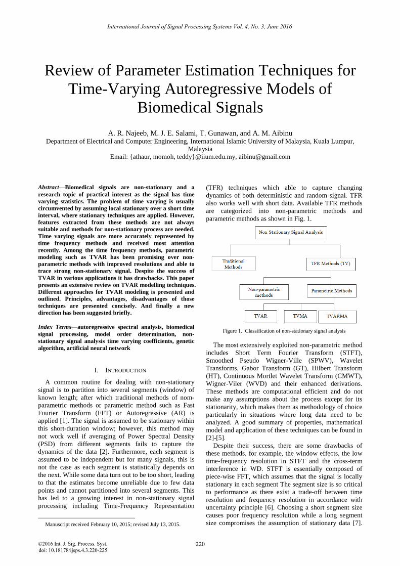
parametric methods as shown in Fig. 1.
Figure 1. Classification of non-stationary signal analysis
The most extensively exploited non-parametric method
includes Short Term Fourier Transform (STFT),
Smoothed Pseudo Wigner-Ville (SPWV), Wavelet
Transforms, Gabor Transform (GT), Hilbert Transform
(HT), Continuous Mortlet Wavelet Transform (CMWT),
Wigner-Viler (WVD) and their enhanced derivations.
These methods are computational efficient and do not
make any assumptions about the process except for its
stationarity, which makes them as methodology of choice
particularly in situations where long data need to be
analyzed. A good summary of properties, mathematical
model and application of these techniques can be found in
[2]-[5].
Despite their success, there are some drawbacks of
these methods, for example, the window effects, the low
time-frequency resolution in STFT and the cross-term
interference in WD. STFT is essentially composed of
piece-wise FFT, which assumes that the signal is locally
stationary in each segment The segment size is so critical
to performance as there exist a trade-off between time
resolution and frequency resolution in accordance with
uncertainty principle [6]. Choosing a short segment size
causes poor frequency resolution while a long segment
size compromises the assumption of stationary data [7].
International Journal of Signal Processing Systems Vol. 4, No. 3, June 2016
©2016 Int. J. Sig. Process. Syst. 220doi: 10.18178/ijsps.4.3.220-225
Although the alternate methods such as WVD yields
good resolutions in both time and frequency for systems
with single components, however when applied on multi-
component signals they produce a lot of artifacts [8].
Consequently, non-parametric methods are limited by
applications and hence are not suitable for broad range of
applications.
The best frequency resolution for non-stationary signal
is obtained by using parametric models where the signal
is fitted into an autoregressive (AR), moving average
(MA) or an autoregressive moving average (ARMA)
model. More parsimonious representation of signals and
higher resolution of time-frequency spectra are
achievable even for a small length of non-stationary
signal using these models. Moreover, the parametric
approaches are able to track relatively fast TV dynamics
and detect multiple TV spectral peaks which may not be
achieved by the non-parametric methods [9]. Un-
availability of long data in biomedical applications such
as EEG, ECG or tumor analysis certainly leads to
parametric methods as preferred method. [10]
Time varying Autoregressive (TVARAR) models have
been investigated by many researchers and received the
most attention in literatues among theexisting parameteric
modeling techniques in last few years [11]. This is
popular assumption for several reasons such as: 1) many
natural signals has underlying autoregressive structure, 2)
any non-stationary signal can be modeled as a AR
process if sufficient model order is selected, 3) estimation
of AR model parameters involves linear system of
equations which can be solved efficiently, 4) the
computational load to calculate the AR model parameters
tend to be less than that for MA or ARMA models.
Despite the success of TVAR in varous applications, it
has few drawback, namely the accuracy of TVAR
coefficient estimation algorithm and the complexity
associated with determining the optimum model order.
Incorrect parametersoften leands to introduction to
artifacts, spurious spectral peaks, false valleys which will
lead to unstable system and consequently this method
will fail. In this paper, methods available to estimate
TVAR parameters are presented and commented.
In next section, we present the TVAR model with its
basic equation. Different TVAR parameter estimation
methods are presented and their computational aspects
are addressed. In Section 3, we compare and discuss
strength and limitation of those algorithms and finally the
conclusion in Section 5.
II. TVAR COEFFICIENT ESTIMATION METHODS
A TVAR process which is driven by a white noise
sequence can be expressed as:
][][][][1
njnynanyp
j
j
(1)
where:
aj[n]; j=1, 2, 3…p are time varying AR coefficients
𝑝 is the model order
][n is zero mean, stationary Gaussian white noise
To model a signal using TVAR parameters, p
and aj[n] is computed. Although p determines the
accuracy of TVAR, many researchers assumes it is
known and estimating only aj[n].
As TVAR coefficient is now a time varying parameter,
popular TIVAR methods developed as Levisohn-Durbin
algorithm or Burg algorithm may not produce desirable
results.
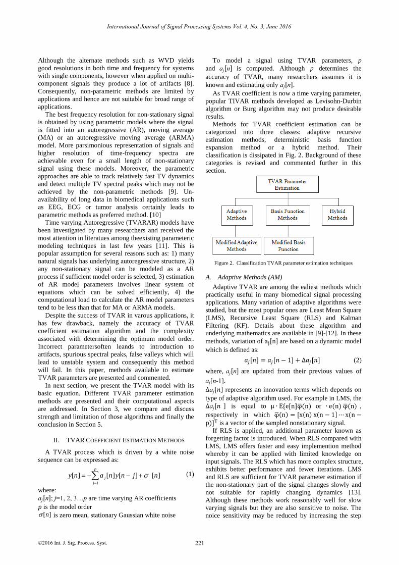
Methods for TVAR coefficient estimation can be
categorized into three classes: adaptive recursive
estimation methods, deterministic basis function
expansion method or a hybrid method. Their
classification is dissipated in Fig. 2. Background of these
categories is revised and commented further in this
section.
Figure 2. Classification TVAR parameter estimation techniques
A. Adaptive Methods (AM)
Adaptive TVAR are among the ealiest methods which
practically useful in many biomedical signal processing
applications. Many variation of adaptive algorithms were
studied, but the most popular ones are Least Mean Square
(LMS), Recursive Least Square (RLS) and Kalman
Filtering (KF). Details about these algorithm and
underlying mathematics are available in [9]-[12]. In these
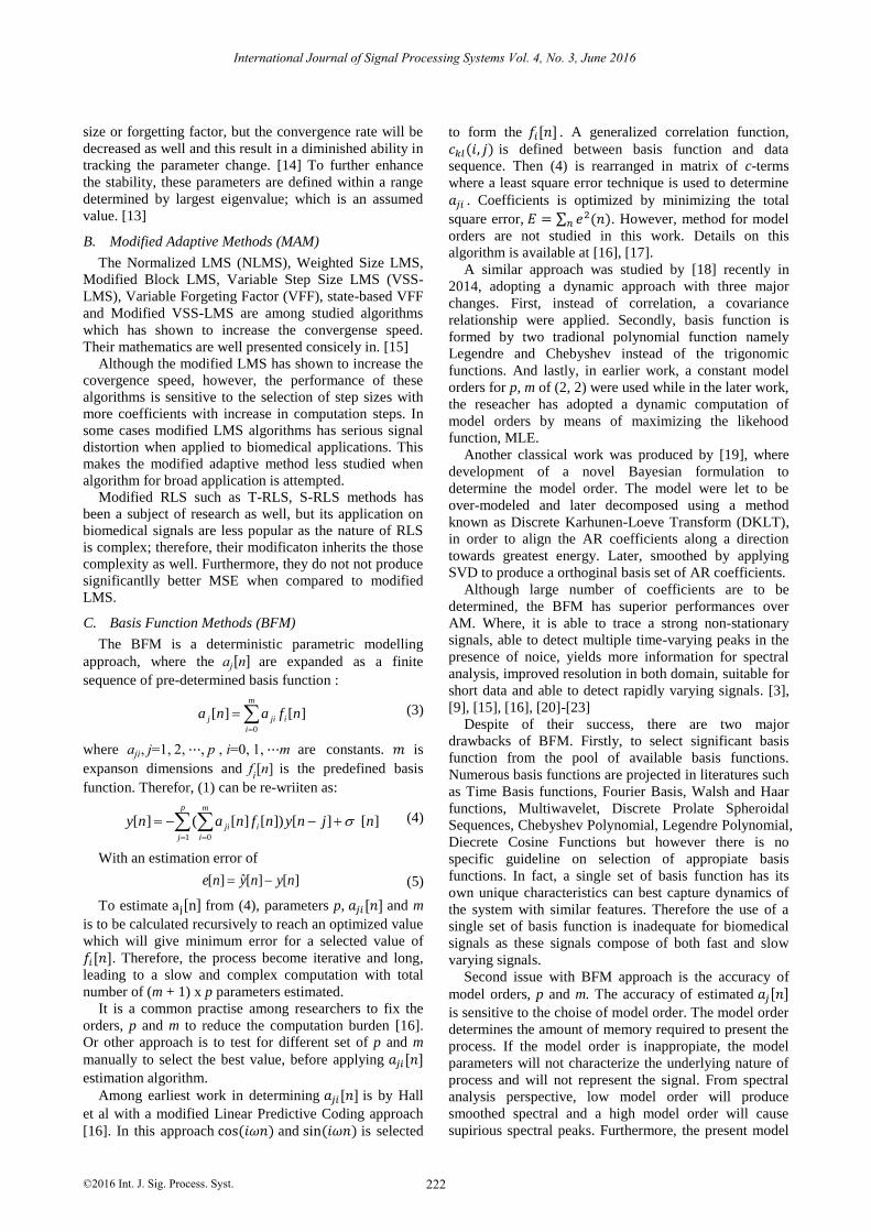
methods, variation of aj[n] are based on a dynamic model
which is defined as:
𝑎𝑗[𝑛] = 𝑎𝑗[𝑛 − 1] + ∆𝑎𝑗[𝑛] (2)
where, aj[n] are updated from their previous values of
aj[n-1].
∆aj[𝑛] represents an innovation terms which depends on
type of adaptive algorithm used. For example in LMS, the
∆aj[𝑛 ] is equal to μ ∙ E{e[n]φ̅(n) or ∙ e(n) φ̅(n) ,
respectively in which φ̅(n) = [x(n) x(n − 1] ⋯ x(n −p)]T is a vector of the sampled nonstationary signal.
If RLS is applied, an additional parameter known as
forgetting factor is introduced. When RLS compared with
LMS, LMS offers faster and easy implemention method
whereby it can be applied with limited knowledge on
input signals. The RLS which has more complex structure,
exhibits better performance and fewer iterations. LMS
and RLS are sufficient for TVAR parameter estimation if
the non-stationary part of the signal changes slowly and
not suitable for rapidly changing dynamics [13].
Although these methods work reasonably well for slow
varying signals but they are also sensitive to noise. The
noice sensitivity may be reduced by increasing the step
International Journal of Signal Processing Systems Vol. 4, No. 3, June 2016
©2016 Int. J. Sig. Process. Syst. 221
size or forgetting factor, but the convergence rate will be
decreased as well and this result in a diminished ability in
tracking the parameter change. [14] To further enhance
the stability, these parameters are defined within a range
determined by largest eigenvalue; which is an assumed
value. [13]
B. Modified Adaptive Methods (MAM)
The Normalized LMS (NLMS), Weighted Size LMS,
Modified Block LMS, Variable Step Size LMS (VSS-
LMS), Variable Forgeting Factor (VFF), state-based VFF
and Modified VSS-LMS are among studied algorithms
which has shown to increase the convergense speed.
Their mathematics are well presented consicely in. [15]
Although the modified LMS has shown to increase the
covergence speed, however, the performance of these
algorithms is sensitive to the selection of step sizes with
more coefficients with increase in computation steps. In
some cases modified LMS algorithms has serious signal
distortion when applied to biomedical applications. This
makes the modified adaptive method less studied when
algorithm for broad application is attempted.
Modified RLS such as T-RLS, S-RLS methods has
been a subject of research as well, but its application on
biomedical signals are less popular as the nature of RLS
is complex; therefore, their modificaton inherits the those
complexity as well. Furthermore, they do not not produce
significantlly better MSE when compared to modified
LMS.
C. Basis Function Methods (BFM)
The BFM is a deterministic parametric modelling
approach, where the aj[n] are expanded as a finite
sequence of pre-determined basis function :
][][ 0
nfana i
m
i
jij
(3)
where aji, j=1, 2, ⋯, p , i=0, 1, ⋯m are constants. 𝑚 is
expanson dimensions and fi[n] is the predefined basis
function. Therefor, (1) can be re-wriiten as:
][][])[][(][1 0
njnynfnanyp
j
m
i
iji
(4)
With an estimation error of
][][ˆ][ nynyne (5)
To estimate aj[n] from (4), parameters p, 𝑎𝑗𝑖[𝑛] and m
is to be calculated recursively to reach an optimized value
which will give minimum error for a selected value of
𝑓𝑖[𝑛]. Therefore, the process become iterative and long,
leading to a slow and complex computation with total
number of (m + 1) x p parameters estimated.
It is a common practise among researchers to fix the
orders, p and m to reduce the computation burden [16].
Or other approach is to test for different set of p and m
manually to select the best value, before applying 𝑎𝑗𝑖[𝑛]
estimation algorithm.
Among earliest work in determining 𝑎𝑗𝑖[𝑛] is by Hall
et al with a modified Linear Predictive Coding approach
[16]. In this approach cos (𝑖𝜔𝑛) and sin (𝑖𝜔𝑛) is selected
to form the 𝑓𝑖[𝑛] . A generalized correlation function,
𝑐𝑘𝑙(𝑖, 𝑗) is defined between basis function and data
sequence. Then (4) is rearranged in matrix of c-terms
where a least square error technique is used to determine
𝑎𝑗𝑖 . Coefficients is optimized by minimizing the total
square error, 𝐸 = ∑ 𝑒2(𝑛)𝑛 . However, method for model
orders are not studied in this work. Details on this
algorithm is available at [16], [17].
A similar approach was studied by [18] recently in
2014, adopting a dynamic approach with three major
changes. First, instead of correlation, a covariance
relationship were applied. Secondly, basis function is
formed by two tradional polynomial function namely
Legendre and Chebyshev instead of the trigonomic
functions. And lastly, in earlier work, a constant model
orders for p, m of (2, 2) were used while in the later work,
the reseacher has adopted a dynamic computation of
model orders by means of maximizing the likehood
function, MLE.
Another classical work was produced by [19], where
development of a novel Bayesian formulation to
determine the model order. The model were let to be
over-modeled and later decomposed using a method
known as Discrete Karhunen-Loeve Transform (DKLT),
in order to align the AR coefficients along a direction
towards greatest energy. Later, smoothed by applying
SVD to produce a orthoginal basis set of AR coefficients.
Although large number of coefficients are to be
determined, the BFM has superior performances over
AM. Where, it is able to trace a strong non-stationary
signals, able to detect multiple time-varying peaks in the
presence of noice, yields more information for spectral
analysis, improved resolution in both domain, suitable for
short data and able to detect rapidly varying signals. [3],
[9], [15], [16], [20]-[23]
Despite of their success, there are two major
drawbacks of BFM. Firstly, to select significant basis
function from the pool of available basis functions.
Numerous basis functions are projected in literatures such
as Time Basis functions, Fourier Basis, Walsh and Haar
functions, Multiwavelet, Discrete Prolate Spheroidal
Sequences, Chebyshev Polynomial, Legendre Polynomial,
Diecrete Cosine Functions but however there is no
specific guideline on selection of appropiate basis
functions. In fact, a single set of basis function has its
own unique characteristics can best capture dynamics of
the system with similar features. Therefore the use of a
single set of basis function is inadequate for biomedical
signals as these signals compose of both fast and slow
varying signals.
Second issue with BFM approach is the accuracy of
model orders, p and m. The accuracy of estimated 𝑎𝑗[𝑛]
is sensitive to the choise of model order. The model order
determines the amount of memory required to present the
process. If the model order is inappropiate, the model
parameters will not characterize the underlying nature of
process and will not represent the signal. From spectral
analysis perspective, low model order will produce
smoothed spectral and a high model order will cause
supirious spectral peaks. Furthermore, the present model
International Journal of Signal Processing Systems Vol. 4, No. 3, June 2016
©2016 Int. J. Sig. Process. Syst. 222
order determination techniques such as Akaike
Information Criterion, Bayesian approach are designed
for conventional AR process such unfit for a TVAR
process. [24]
D. Modified Basis Function Methods (MBFM)
MBFM methods were introduced to overcome the
limitations of BFM which includes dynamic computation
of model orders or to study on optimized basis functions.
Optimal Parameter Search Algorithm was proposed in
[24] where the authors accurately determine the model
order and extract the significant model terms by
discriminating irrelevant basis sequence. It has been
shown that this method works well for overparametrized,
corrupted signals and is also applicable for linear and
non-linear system. Then irrelvant basis sequence where
removed pool of candidate vectors and a liner
independent matrix were formed before least square
method is applied. A projecton distance is calculated to
compute model orders p and m. Although this proved
better performances, but more parameters were
introduced and it becomes increasingly complex at each
level of n. The same methods were studied again using
multiple set of basis function [12] with similar success
but again with huge number of coeffiecients and
intermediate parameters were used. Accuracy of model order may also increased is by
adopting forward and backward (FB) TVAR. A system
with such approach is flexible and has superior
performance over the model using only causal (forward)
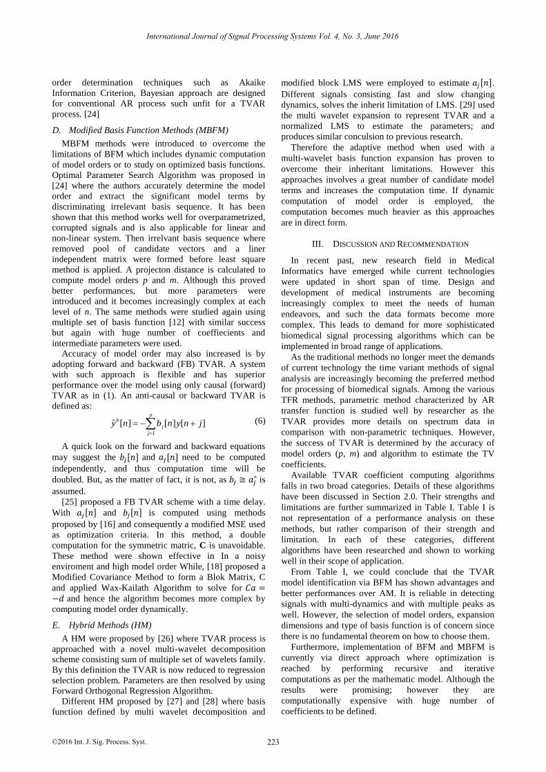
TVAR as in (1). An anti-causal or backward TVAR is
defined as:
][][][ˆ1
jnynbnyp
j
j
b
(6)
A quick look on the forward and backward equations
may suggest the 𝑏𝑗[𝑛] and 𝑎𝑗[𝑛] need to be computed
independently, and thus computation time will be
doubled. But, as the matter of fact, it is not, as 𝑏𝑗 ≅ 𝑎𝑗∗ is
assumed.
[25] proposed a FB TVAR scheme with a time delay.
With 𝑎𝑗[𝑛] and 𝑏𝑗[𝑛] is computed using methods
proposed by [16] and consequently a modified MSE used
as optimization criteria. In this method, a double
computation for the symmetric matric, C is unavoidable.
These method were shown effective in In a noisy
enviroment and high model order While, [18] proposed a
Modified Covariance Method to form a Blok Matrix, C
and applied Wax-Kailath Algorithm to solve for 𝐶𝑎 =−𝑑 and hence the algorithm becomes more complex by
computing model order dynamically.
E.
A HM were proposed by [26] where TVAR process is
approached with a novel multi-wavelet decomposition
scheme consisting sum of multiple set of wavelets family.
By this definition the TVAR is now reduced to regression
selection problem. Parameters are then resolved by using
Forward Orthogonal Regression Algorithm.
Different HM proposed by [27] and [28] where basis
function defined by multi wavelet decomposition and
modified block LMS were employed to estimate 𝑎𝑗[𝑛].
Different signals consisting fast and slow changing
dynamics, solves the inherit limitation of LMS. [29] used
the multi wavelet expansion to represent TVAR and a
normalized LMS to estimate the parameters; and
produces similar conculsion to previous research.
Therefore the adaptive method when used with a
multi-wavelet basis function expansion has proven to
overcome their inheritant limitations. However this
approaches involves a great number of candidate model
terms and increases the computation time. If dynamic
computation of model order is employed, the
computation becomes much heavier as this approaches
are in direct form.
III. DISCUSSION AND RECOMMENDATION
In recent past, new research field in Medical
Informatics have emerged while current technologies
were updated in short span of time. Design and
development of medical instruments are becoming
increasingly complex to meet the needs of human
endeavors, and such the data formats become more
complex. This leads to demand for more sophisticated
biomedical signal processing algorithms which can be
implemented in broad range of applications.
As the traditional methods no longer meet the demands
of current technology the time variant methods of signal
analysis are increasingly becoming the preferred method
for processing of biomedical signals. Among the various
TFR methods, parametric method characterized by AR
transfer function is studied well by researcher as the
TVAR provides more details on spectrum data in
comparison with non-parametric techniques. However,
the success of TVAR is determined by the accuracy of
model orders (p, m) and algorithm to estimate the TV
coefficients.
Available TVAR coefficient computing algorithms
falls in two broad categories. Details of these algorithms
have been discussed in Section 2.0. Their strengths and
limitations are further summarized in Table I. Table I is
not representation of a performance analysis on these
methods, but rather comparison of their strength and
limitation. In each of these categories, different
algorithms have been researched and shown to working
well in their scope of application.
From Table I, we could conclude that the TVAR
model identification via BFM has shown advantages and
better performances over AM. It is reliable in detecting
signals with multi-dynamics and with multiple peaks as
well. However, the selection of model orders, expansion
dimensions and type of basis function is of concern since
there is no fundamental theorem on how to choose them.
Furthermore, implementation of BFM and MBFM is
currently via direct approach where optimization is
reached by performing recursive and iterative
computations as per the mathematic model. Although the
results were promising; however they are
computationally expensive with huge number of
coefficients to be defined.
International Journal of Signal Processing Systems Vol. 4, No. 3, June 2016
©2016 Int. J. Sig. Process. Syst. 223
Hybrid Methods (HM)
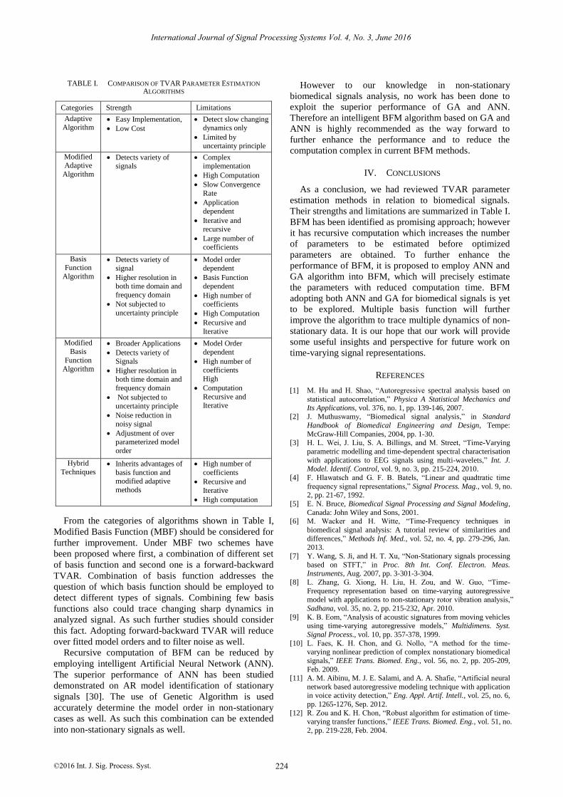
TABLE I. COMPARISON OF TVAR PARAMETER ESTIMATION
ALGORITHMS
Categories Strength Limitations
Adaptive Algorithm
Easy Implementation,
Low Cost
Detect slow changing dynamics only
Limited by uncertainty principle
Modified Adaptive
Algorithm
Detects variety of signals
Complex implementation
High Computation
Slow Convergence
Rate
Application
dependent
Iterative and recursive
Large number of coefficients
Basis Function
Algorithm
Detects variety of signal
Higher resolution in both time domain and
frequency domain
Not subjected to
uncertainty principle
Model order dependent
Basis Function dependent
High number of coefficients
High Computation
Recursive and
Iterative
Modified
Basis
Function Algorithm
Broader Applications
Detects variety of Signals
Higher resolution in both time domain and
frequency domain
Not subjected to uncertainty principle
Noise reduction in noisy signal
Adjustment of over parameterized model
order
Model Order
dependent
High number of coefficients
High
Computation
Recursive and Iterative
Hybrid
Techniques Inherits advantages of
basis function and modified adaptive
methods
High number of
coefficients
Recursive and
Iterative
High computation
From the categories of algorithms shown in Table I,
Modified Basis Function (MBF) should be considered for
further improvement. Under MBF two schemes have
been proposed where first, a combination of different set
of basis function and second one is a forward-backward
TVAR. Combination of basis function addresses the
question of which basis function should be employed to
detect different types of signals. Combining few basis
functions also could trace changing sharp dynamics in
analyzed signal. As such further studies should consider
this fact. Adopting forward-backward TVAR will reduce
over fitted model orders and to filter noise as well.
Recursive computation of BFM can be reduced by
employing intelligent Artificial Neural Network (ANN).
The superior performance of ANN has been studied
demonstrated on AR model identification of stationary
signals [30]. The use of Genetic Algorithm is used
accurately determine the model order in non-stationary
cases as well. As such this combination can be extended
into non-stationary signals as well.
However to our knowledge in non-stationary
biomedical signals analysis, no work has been done to
exploit the superior performance of GA and ANN.
Therefore an intelligent BFM algorithm based on GA and
ANN is highly recommended as the way forward to
further enhance the performance and to reduce the
computation complex in current BFM methods.
IV. CONCLUSIONS
As a conclusion, we had reviewed TVAR parameter
estimation methods in relation to biomedical signals.
Their strengths and limitations are summarized in Table I.
BFM has been identified as promising approach; however
it has recursive computation which increases the number
of parameters to be estimated before optimized
parameters are obtained. To further enhance the
performance of BFM, it is proposed to employ ANN and
GA algorithm into BFM, which will precisely estimate
the parameters with reduced computation time. BFM
adopting both ANN and GA for biomedical signals is yet
to be explored. Multiple basis function will further
improve the algorithm to trace multiple dynamics of non-
stationary data. It is our hope that our work will provide
some useful insights and perspective for future work on
time-varying signal representations.
REFERENCES
[1] M. Hu and H. Shao, “Autoregressive spectral analysis based on
statistical autocorrelation,” Physica A Statistical Mechanics and
Its Applications, vol. 376, no. 1, pp. 139-146, 2007. [2] J. Muthuswamy, “Biomedical signal analysis,” in Standard
Handbook of Biomedical Engineering and Design, Tempe:
McGraw-Hill Companies, 2004, pp. 1-30. [3] H. L. Wei, J. Liu, S. A. Billings, and M. Street, “Time-Varying
parametric modelling and time-dependent spectral characterisation
with applications to EEG signals using multi-wavelets,” Int. J. Model. Identif. Control, vol. 9, no. 3, pp. 215-224, 2010.
[4] F. Hlawatsch and G. F. B. Batels, “Linear and quadtratic time
frequency signal representations,” Signal Process. Mag., vol. 9, no. 2, pp. 21-67, 1992.
[5] E. N. Bruce, Biomedical Signal Processing and Signal Modeling,
Canada: John Wiley and Sons, 2001. [6] M. Wacker and H. Witte, “Time-Frequency techniques in
biomedical signal analysis: A tutorial review of similarities and
differences,” Methods Inf. Med., vol. 52, no. 4, pp. 279-296, Jan.
2013.
[7] Y. Wang, S. Ji, and H. T. Xu, “Non-Stationary signals processing
based on STFT,” in Proc. 8th Int. Conf. Electron. Meas. Instruments, Aug. 2007, pp. 3-301-3-304.
[8] L. Zhang, G. Xiong, H. Liu, H. Zou, and W. Guo, “Time-
Frequency representation based on time-varying autoregressive model with applications to non-stationary rotor vibration analysis,”
Sadhana, vol. 35, no. 2, pp. 215-232, Apr. 2010.
[9] K. B. Eom, “Analysis of acoustic signatures from moving vehicles using time-varying autoregressive models,” Multidimens. Syst.
Signal Process., vol. 10, pp. 357-378, 1999.
[10] L. Faes, K. H. Chon, and G. Nollo, “A method for the time-varying nonlinear prediction of complex nonstationary biomedical
signals,” IEEE Trans. Biomed. Eng., vol. 56, no. 2, pp. 205-209,
Feb. 2009. [11] A. M. Aibinu, M. J. E. Salami, and A. A. Shafie, “Artificial neural
network based autoregressive modeling technique with application in voice activity detection,” Eng. Appl. Artif. Intell., vol. 25, no. 6,
pp. 1265-1276, Sep. 2012.
[12] R. Zou and K. H. Chon, “Robust algorithm for estimation of time-varying transfer functions,” IEEE Trans. Biomed. Eng., vol. 51, no.
2, pp. 219-228, Feb. 2004.
International Journal of Signal Processing Systems Vol. 4, No. 3, June 2016
©2016 Int. J. Sig. Process. Syst. 224
[13] S. Elouaham, R. Latif, and A. Dliou, “Parametric and non parametric time-frequency analysis of biomedical signals,” Int. J.
Adv. Comput. Sci. Appl., vol. 4, no. 1, pp. 74-79, 2013.
[14] F. Shiman, S. H. Safavi, F. M. Vaneghi, M. Oladazimi, M. J. Safari, and F. Ibrahim, “EEG feature extraction using parametric
and non-parametric models,” in Proc. IEEE-EMBS International
Conference on Biomedical and Health Informatics, Hong Kong, 2012, vol. 25, pp. 66-70.
[15] E. Eweda, “Advances in nonstationary adaptive signal processing,”
in Proc. Thirteenth National Radio Science Conference, Cairo, 1996, pp. 61-82.
[16] M. G. Hall, A. V. Oppenheim, and A. S. Willsky, “Time-Varying
parametric modeling of speech,” Signal Processing, vol. 5, no. 049, pp. 267-285, 1983.
[17] G. R. S. Reddy, R. Rao, and C. V. R. College, “Performance
analysis of basis functions in TVAR model,” Int. J. Signal Process. Image Process. Pattern Recognit., vol. 7, no. 3, pp. 317-338, 2014.
[18] G. R. S. Reddy and R. Rao, “Instantaneous frequency estimation
based on time-varying auto regressive model and WAX-kailath algorithm,” An Int. J. Signal Process., vol. 8, no. 4, pp. 43-66,
2014.
[19] J. J. Rajan and P. J. W. Rayner, “Generalize feature extraction for time varying autoregressive models,” IEEE Trans. on Signal
Processing, vol. 44, no. 10, Oct. 1996.
[20] M. J. Cassidy and W. D. Penny, “Bayesian nonstationary autoregressive models for biomedical signal analysis,” IEEE
Trans. Biomed. Eng., vol. 49, no. 10, pp. 1142-1152, Oct. 2002.
[21] Y. Li, H. Wei, S. A. Billings, P. Sarrigiannis, S. A. Billings, and P. G. Sarrigiannis, “Time-Varying model identification for time-
frequency feature extraction from EEG data,” J. Neurosci.
Methods, vol. 196, no. 1021, pp. 1-13, 2011. [22] R. Zou, H. Wang, and K. H. Chon, “A robust time-varying
identification algorithm using basis functions,” Ann. Biomed. Eng.,
vol. 31, no. 7, pp. 840-853, Jul. 2003. [23] G. R. S. Reddy, R. Rao, and C. V. R. College, “Non-Stationary
signal analysis using TVAR model,” Int. J. Signal Process. Image
Process. Pattern Recognit., vol. 7, no. 2, pp. 411-430, 2014. [24] A. H. Costa and S. Hengstler, “Adaptive time-frequency analysis
based on autoregressive modeling,” Signal Processing, vol. 91, no. 4, pp. 740-749, Apr. 2011.
[25] C. Sodsri, “Time-Varying autoregressive modelling for
nonstationary acoustic signal and its frequency analysis,” Ph.D. thesis, The Pennsylavania State University, Dec. 2003.
[26] K. H. Chon, H. Zhao, R. Zou, and K. Ju, “Multiple time-varying
dynamic analysis using multiple sets of basis functions,” IEEE Trans. Biomed. Eng., vol. 52, no. 5, pp. 956-960, May 2005.
[27] Y. Li, H. L. Wei, S. A. Billings, and H. Wei, “Time-Varying
signal processing using multi-wavelet basis functions and a
modified block least mean square algorithm,” Research Report, ACSE Research Report No. 998, Automatic Control and Systems
Engineering, University of Sheffield, pp. 1-17, 2009.
[28] Y. Li, H. Wei, and S. A. Billings, “Identification of time-varying systems using multi-wavelet basis functions,” IEEE Trans.
Control Syst. Technol., vol. 19, no. 3, pp. 656-663, May 2011.
[29] S. N. Mate and A. B. Patil, “Identification of time varying system using recursive estimation approach and wavelet based recursive
estimation approach,” Int. J. Eng. Sci. Innov. Technol., vol. 2, no.
3, pp. 526-532, 2013. [30] J. Tian, M. Juhola, and T. Grönfors, “AR parameter estimation by
a feedback neural network,” Comput. Stat. Data Anal., vol. 25, no.
1, pp. 17-24, Jul. 1997.
Athaur Rahman Bin Najee
Engineering, Department of Electrical and Computer Engineering. He carries his research under supervision of Prof. Dr. Momoh Jimoh E.
Salami and Dr. Teddy Gunawan. Athaur Rahman Bin Najeeb received
his Master of Science in Electrical and Computer Engineering from IIUM in 2008. His research interests focus on Biomedical Signals
Processing, Image Processing.
Prof. Dr. Momoh Jimoh Eyiomika Salami is Professor of Signal and
Image Processing, International Islamic University Malaysia Professor
at the Department of Mechatronics. He has authored/co-authored more than 100 publications in both local and international journals and
conference proceedings as well as being one of the contributors. He had
contributed a chapter in recently published book entitled “The Mechatronics Handbook” edited by Prof. Bishop. His research interests
include Digital Signal and Image Processing, Intelligent Control
Systems Design and instrumentation. Prof. Momoh is a senior member of IEEE.
Dr. Teddy Gunawan obtained his M. Eng from School of Computer Engineering, Nanyang Technological University in 1999 and his PhD in
Electrical Engineering from School of Electrical Engineering and
Telecommunications He is a Senior Member of IEEE. His research interests are Speech and audio signal processing, Genomic signal
processing, Biomedical instrumentation and signal processing, Image processing and computer
Dr. Abiodun Musa Aibinu is Associate Professor and a technical expert in emerging application of Signal Processing. He obtained his
PhD in Signal Processing from IIUM in 2011. Currently he is Director,
at Center for Open Distance and e-Learning (CODEL), FUT Minna. His research interests include: Biomedical Signal, Processing; Digital Image
Processing; Instrumentation and Measurements; Telecommunication
system Design and Digital System Design.
International Journal of Signal Processing Systems Vol. 4, No. 3, June 2016
©2016 Int. J. Sig. Process. Syst. 225
b is a PhD student in Faculty of