STOCHASTIC MODELLING OF TIME LAG FOR SOLVENT … · (PEMODELAN STOKASTIK DENGAN MASALENGAHAN BAGI...
13
JurnalKaryaAsliLorekanAhliMatematik Vol. 4 No.1 (2011) Page 13 - 25 Jurnal Karya Asli Lorekan Ahli Matematik © 2010 JurnalKaryaAsliLorekanAhliMatematik Published by PustakaAman Press Sdn. Bhd. STOCHASTIC MODELLING OF TIME LAG FOR SOLVENT PRODUCTION BY C. ACETOBUTYLICUM P262 (PEMODELAN STOKASTIK DENGAN MASALENGAHAN BAGI PENGHASILAN PELARUT OLEH C. ACETOBUTYLICUM P262) 1 Norhayati Rosli, 1 Arifah Bahar, 1 Yeak Su Hoe, 1 Haliza Abd. Rahman and 2 Madihah MohdSalleh 1 Department of Mathematics, Faculty Science, UniversitiTeknologi Malaysia, 81310, Skudai, Johor 2 Faculty of Bioscience and Bioengineering, UniversitiTeknologi Malaysia, 81310 Skudai, Johor 1 [email protected] Abstract :This work is carried out to model jointly time delay and unknown disturbances of gelatinised sago starch to solvent production by C. acetobutylicum P262. The proposed model of C. acetobutylicum P262 proliferation is formulated as stochastic delay logistic model. Moreover, Luedeking-Piret equations were used to model the solvent production of acetone and butanol by C. acetobutylicum P262, whose number of living cell, ) (t x is subjected to time delay and beyond deterministic behaviour. The strong solution of the resulting models was simulated numerically via numerical method of Euler-Maruyama (EM). Their respective root mean square errors (RMSE) were calculated by comparing the simulated and experimental data so that the prediction quality of the model can be assessed. Abstrak :Penyelidikan ini dijalankan bagi memodelkan lengahan masa dan hingar rawak yang terdapat dalam proses penghasilan pelarut oleh C. acetobutylicum P262. Model yang dicadangkan bagi mengkaji kadar pertumbuhan sel C. acetobutylicum P262 adalah stokastik logistic model yang melibatkan masa lengahan. Persamaan Luedeking-Piret digunakan untuk memodelkan pembentukan pelarut acetondanbutanol oleh C. acetobutylicum P262. Kepekatan sel hidup, ) (t x tertakluk kepada masa lengahan dan bukan lagi tertentu. Penyelesaian hampiran bagi model tersebut dihitung menggunakan kaedah berangka Euler-Maruyama (EM). Ralat min punca kuasadua dihitung bagi menentukan kepersisan model yang dibentuk. Keywords:Stochastic delay differential equations (SDDEs), Delay Differential Equations (DDEs), Stochastic Ordinary Differential Equations (SODEs), Euler-Maruyama (EM). 1. Introduction Modelling of physical phenomena and biological system using ordinary differential equations (ODEs) and stochastic ordinary differential equations (SODEs) has become an intensive research over last few years. In both types of equations the unknown function and its derivatives are evaluated at the same instant time, t. However, it was generally acknowledge that many of the natural phenomena around us do not have an immediate effect from the moment of their occurrence. For instance, the growth of the microbe is not instantaneous but responds only after some time lag, 0 . In such cases, ODEs and SODEs which are simply depending on the present state are inadequate to describe the process that involves time delay. The modelling of such phenomena, leading to what is called delay differential equations (DDEs) and stochastic delay differential equations (SDDEs). Indeed, DDEs are unsatisfactory to model the process with the presence of random effects. Definitely the dynamical systems whose evolution in time is governed by uncontrolled fluctuationsas well as the unknown function is depending on its past history can often be modelled via SDDEs.
Transcript of STOCHASTIC MODELLING OF TIME LAG FOR SOLVENT … · (PEMODELAN STOKASTIK DENGAN MASALENGAHAN BAGI...
JurnalKaryaAsliLorekanAhliMatematik Vol. 4 No.1 (2011) Page 13 - 25
Jurnal
Karya Asli Lorekan
Ahli Matematik
© 2010 JurnalKaryaAsliLorekanAhliMatematik
Published by PustakaAman Press Sdn. Bhd.
STOCHASTIC MODELLING OF TIME LAG FOR SOLVENT
PRODUCTION BY C. ACETOBUTYLICUM P262
(PEMODELAN STOKASTIK DENGAN MASALENGAHAN BAGI
PENGHASILAN PELARUT OLEH C. ACETOBUTYLICUM P262)
1Norhayati Rosli, 1Arifah Bahar, 1Yeak Su Hoe, 1Haliza Abd. Rahman and 2Madihah
MohdSalleh 1Department of Mathematics, Faculty Science,
UniversitiTeknologi Malaysia,
81310, Skudai, Johor 2Faculty of Bioscience and Bioengineering,
UniversitiTeknologi Malaysia,
81310 Skudai, Johor [email protected]
Abstract :This work is carried out to model jointly time delay and unknown disturbances of gelatinised sago
starch to solvent production by C. acetobutylicum P262. The proposed model of C. acetobutylicum P262
proliferation is formulated as stochastic delay logistic model. Moreover, Luedeking-Piret equations were used to
model the solvent production of acetone and butanol by C. acetobutylicum P262, whose number of living cell,
)(tx is subjected to time delay and beyond deterministic behaviour. The strong solution of the resulting models
was simulated numerically via numerical method of Euler-Maruyama (EM). Their respective root mean square
errors (RMSE) were calculated by comparing the simulated and experimental data so that the prediction quality
of the model can be assessed.
Abstrak :Penyelidikan ini dijalankan bagi memodelkan lengahan masa dan hingar rawak yang terdapat dalam
proses penghasilan pelarut oleh C. acetobutylicum P262. Model yang dicadangkan bagi mengkaji kadar
pertumbuhan sel C. acetobutylicum P262 adalah stokastik logistic model yang melibatkan masa lengahan.
Persamaan Luedeking-Piret digunakan untuk memodelkan pembentukan pelarut acetondanbutanol oleh C.
acetobutylicum P262. Kepekatan sel hidup, )(tx tertakluk kepada masa lengahan dan bukan lagi tertentu.
Penyelesaian hampiran bagi model tersebut dihitung menggunakan kaedah berangka Euler-Maruyama (EM).
Ralat min punca kuasadua dihitung bagi menentukan kepersisan model yang dibentuk.
Keywords:Stochastic delay differential equations (SDDEs), Delay Differential Equations (DDEs), Stochastic
Ordinary Differential Equations (SODEs), Euler-Maruyama (EM).
1. Introduction
Modelling of physical phenomena and biological system using ordinary differential equations
(ODEs) and stochastic ordinary differential equations (SODEs) has become an intensive research over
last few years. In both types of equations the unknown function and its derivatives are evaluated at the
same instant time, t. However, it was generally acknowledge that many of the natural phenomena
around us do not have an immediate effect from the moment of their occurrence. For instance, the
growth of the microbe is not instantaneous but responds only after some time lag, 0 . In such
cases, ODEs and SODEs which are simply depending on the present state are inadequate to describe
the process that involves time delay. The modelling of such phenomena, leading to what is called
delay differential equations (DDEs) and stochastic delay differential equations (SDDEs). Indeed,
DDEs are unsatisfactory to model the process with the presence of random effects. Definitely the
dynamical systems whose evolution in time is governed by uncontrolled fluctuationsas well as the
unknown function is depending on its past history can often be modelled via SDDEs.
Jurnal KALAM Vol. 4, No. 1, Page 13 - 25
14
Our main concern in this paper is to model jointly time delay and unknown disturbances of
gelatinised sago starch to solvent production by C.acetobutylicumP262 of batch process. In typical
batch fermentation, there are two important features that control the mechanism of the process namely
time delays and the system is continually subjected to the effects of random or uncontrolled
fluctuations which are referred as noise. The presence of time delay is a consequence of the simple
fact that initially, microbial are in the process of adapting themselves to the new environment, thus no
growth occur. They are in the situation to synthesis the new enzymes in response to change in the
availability of substitutable substrates [2]. The microbe in this position is said to be in a lag phase. At
the end of the lag phase, the population of microorganisms is well-adjusted to the new environment,
cells multiply rapidly and cell mass doubles regularly with time. Microbe subsequently enters a period
called an exponential phase. As time evolves, the system is subjected to an intrinsic variability of the
competing within species and deviations from exponential growth arise. It happens as a result of the
nutrient level and toxinconcentration achieves a value which unable to sustain the maximum growth
rate. This phase is recognized as a stationary phase. By taking into account all the phases involve in
batch fermentation, modellers should aware that mathematical models for the dynamic of this process
take the form of SDDEs. In many problems, analytical solution for SDDEs is not available and
numerical methods provide a suitable way to approximate their solutions. In the present article,the
strong solution of the proposed model is approximated via EM method. It was [4] who proposed a
numerical method of EM for SDDE. This method has order of convergence of 0.5, yet it is the
simplest to be implemented in C.
This paper is organized as follows; Section 2.0 reviewed the latest mathematical model of
ODEs, DDEs and SODEs used to describe the cell growth and solvent production of batch
fermentation. Then, we incorporate a slow microbial adaptation and unknown disturbances of the
system via SDDE model. A description of numerical methods and numerical algorithm for SDDEs is
carried out in Section 3.0. We present the values of kinetic parameter model in Section 4.0 and the
results of solvent production by C. acetobutylicumP262 are demonstrated. Lastly, the root mean
square error (RMSE) is computed in order to assess the validity of the stochastic model with time lag.
2. Reviews on Mathematical Modelling of Cell Growth & Solvent Production
The classical logistic ODE used to describe the cell growth of C. acetobutylicum P262 is given
below
],[),()(
1)(
max
max Tttxx
tx
dt
tdx
(1)
The constant maxx denotes the maximum cell concentration (g/L), max correspond to maximum
specific growth rate (h-1) and T is the terminal point of time )(h . In natural environment maxx is
limiting population determined by carrying capacity of the environment. This model has been used by
[18] to model the cell growth of C. acetobutylicum in batch system. The production of acetone and
butanol were formulated as Luedeking-Piret equation of
Acetone: xbdt
dxa
dt
dA
(2)
Butanol: xedt
dxc
dt
dB
(3)
where
x concentration of cell mass (g/L),
A = acetone concentration (g/L)
a = growth associated coefficient for acetone formation (g substrate/g cell)
b = non-growth associated coefficient for acetone formation (g substrate/g cell)
B = butanol concentration (g/L)
Norhayatiet. al.
15
c = growth associated coefficient for butanol formation (g substrate/g cell)
e = non-growth associated coefficient for butanol formation (g substrate/g cell)
The differential equations (1), (2) and (3) had been used to model the solvent production by C.
acetobutylicum in [9]. As aforementioned in [9], the production of acetone and butanol was non-
growth associated system. Therefore, the values of growth associated coefficient for product
formation was zero. The exact solution of (1) and Luedeking-Piret equations of (2) and (3) can be
written in the following form
Cell growth:
)exp(1
)exp()(
max
0
max
maxmax
tx
x
txtx
(4)
Product formation
Acetone:
t
t
dssxbtAtA
0
)()()( 0 (5)
Butanol:
t
t
dssxetBtB
0
)()()( 0 (6)
where )(),( 000 tAtxx and )( 0tB represent the initial cell, acetone and butanol concentration
respectively. It is reasonable to model the cell growth via DDEs by assumption that initially cells are
inactive and once it is activated the cell division is not instantaneous [3]. Early attempt to model the
population growth using logistic DDE has been made in [6]. He proposed a classical delay logistic
model by assuming biological self-regulatory reaction represented by the factor max
)(1
x
tx in (1) is not
instantaneous but responds only after some time lag, 0 . The original motivation of [6] by
introducing time delay in classical logistic ODE is to model the oscillations observed in Daphnia
populations, on the ground that fertility of the pathogenetic female influenced by the density of past
population. An obvious distinction between DDEs and ODEs is in specifying the initial value, )( 0tx .
For DDE, it is not enough to determine the solution for 0t by having )( 0tx alone. We need to have
initial function, to specify the history of )(tx for ]0,[ t . Thus, the corresponding classical
logistic DDE of (1) is
]0,[),()(
],[),()(
1)('max
max
tttx
Tttxx
txtx
(7)
The time delay models the length of the time period between the initial time and maturing
time wherein the division of the cell begins. The presence of internal and external noise in batch
system ultimately linked with the theory of SODEs. The deterministic model of (1) and (7) do not
accommodate random variations of metabolism. An alternative stochastic model would result from
the hypothesis that the process itself is not smooth. The cell growth of C. acetobutylicum P262 is
subjected to a variety of internal and external influences, which change over time. Therefore, it is
necessary to add suitable system variability to the deterministic model (1). In [1] the parameter max
max
x
is allowed to vary randomly by introducing a white noise perturbation that is
Jurnal KALAM Vol. 4, No. 1, Page 13 - 25
16
,)(
dt
tdWbb (8)
where max
max
xb
, is a diffusion coefficient and )(tW is a one dimensional stochastic process
having scalar Wiener process components that is the increment )()()( tWttWtW are
independent Gaussian random variables with mean zero and variance the increment of the time, t .
Model (1) with perturbation (8) is an Itô SODE of the following
),()()()(
1)( 2
max
max tdWtxdttxx
txtdx
(9)
or more accurately as an integral equation
.)()()()(
1)(0
2
0 max
max0
TT
sdWsxdssxx
sxxtx (10)
The second integral in (6) is stochastic integral with respect to a Wiener process, )(tW . The
Wiener process is nowhere differentiable and its continuous sample path are not bounded variation.
So, it cannot be interpreted as Riemann-Stieltjes integral. The stochastic integrals can be interpreting
either as Itô or Stratonovich integral depending on the evaluation points of the integrand. Model (9) is
formulated in [13] to model cell proliferation of the microbe in batch fermentation. The strong
solution of SODE (9) was approximated using EM. Model (9) can be transformed into Stratonovich
form and vice-versa by means of the following formula
).,(),(2
1),(),( tttt xt
x
gxtgxtfxtf
(11)
where ),( txtf is drift coefficient and ),( txtg is known as diffusion coefficient. By employing (11) to
drift coefficient in (9) we obtain the stochastic model in Stratonovich form of
),()()()()(
1)( 232
max
max tdWtxdttxtxx
txtdx
(12)
or in the integral form
.)()()()()(
1)(0
2
0
32
max
max0
TT
sdWsxdssxsxx
sxxtx (13)
The symbol is used to indicate the Stratonovich SODE (i.e. )(tdW ). SODE (12) has been
formulated in [17] to model the cell growth in batch culture and the strong solution of SODE is
simulated via SRK2. In the acetone-butanol biosynthesis process by C. acetobutylicum P262, a more
sophisticated insight into physical phenomena may be achieved if we consider problems with both
time-lag and assume that the observed biological system operate in noisy environment. In such a case,
it is practical to model the cell division in batch culture via SDDE. Therefore, the model we derive in
the present article is in the form of (13) with random perturbation to max
max
x
. It means that, the
mathematical model of SDDE is formulated to describe the cell growth of C. acetobutylicumP262.
SDDE can be approached either as SODE with added delay or DDE with noise [14]. The second
approach shall be considered here. We assume that our model is in autonomous form. Therefore, a
general formulation of autonomous SDDE is
0,],[),()(
],[),())(),(())(),(()(
0
ttttx
TttdWtxtxgdttxtxftdx (14)
Norhayatiet. al.
17
or in integral form it can formulated rigorously as
0,,),()(
,,)()(),())(),(()(
0
00
ttttx
TtsdWsxsxgdssxsxftx
t
t
t
t
(15)
where RRRf : and RRRg : . The functions gf and need to satisfy the local Lipchitz
condition and linear growth condition in order to ensure the existence and uniqueness solution [11]. In
applied problems the initial function, )(t for 0 t is found experimentally and also may be
determined from another equation without deviating argument. For our purpose )(t is determined
experimentally. Let we have the delay logistic equation of (13) in the form of
Tttxtxxx
tx ,,' max
max
max
(16)
Then, perturbation through parameter
dt
tdW
xx
max
max
max
max , leading to the following differential
equation
).()()()()(
1)(max
max tdWtxtxdttxx
txtdx
(17)
Thus, a simplified batch fermentation kinetic model for cell growth of C. acetobutylicumP262 is in the
form of (17). The mathematical model of solvent production in terms of )(tx are given as below
Acetone )(txbdt
dA (18)
Butanol )(txddt
dB (19)
where )(tx is subjected to time delay and no longer deterministic. Kinetic parameter model of
db,,max and need to be estimated.
3. Euler-Maruyama Scheme and Numerical Coding
We have considered strong Euler-Maruyama approximations with a fixed step size, h on the
interval ],0[ T , for NnhntN
Th n ,,1,)1(, . We assumed that, there is an integer
number N such that the delay can be expressed in terms of the step size hN . For SDDE (14),
the Euler-Maruyama scheme has the following form
)))((),(())(),(()()( 1 nnnnnnn Wtxtxgtxtxbhtxtx (20)
with ),()( 1 nnn tWtWW denoting independent ),0( hN distributed Gaussian random
variables. The Euler discretization for the process given in (17) looks like
)()(1)()(max
max1 nNnnn
Nn
nn Wxxhtxx
xtxtx
(21)
We generate a code to simulate the solution of discretization process (15) using the language of C.
The resulting algorithm is presented below;
Jurnal KALAM Vol. 4, No. 1, Page 13 - 25
18
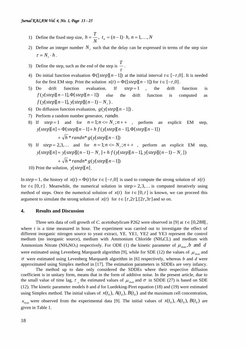
1) Define the fixed step size, NnhntN
Th n ,,1,)1(,
2) Define an integer number N such that the delay can be expressed in terms of the step size
hN .
3) Define the step, such as the end of the step is
T.
4) Do initial function evaluation ])1][([ nstep at the initial interval ]0,[ t . It is needed
for the first EM step. Print the solution ])1][([)( nsteptx for ]0,[ t .
5) Do drift function evaluation. If 1step , the drift function is
])1][[],1][[( nstepnstepyf else the drift function is computed as
))1][([],1][[( Nnstepynstepyf .
6) Do diffusion function evaluation, ])1][[( nstepyg .
7) Perform a random number generator, randn.
8) If 1step and for nNnn ;;1 , perform an explicit EM step,
])1][[(**
)]1][[],1][[(]1][[]][[
nstepygrandnh
nstepnstepyfhnstepnstepy
9) If ,3,2step and for nNnn ;;1 , perform an explicit EM step,
])1][[(**
)])1][([],1][[(])1][([]][[
nstepygrandnh
NnstepynstepyfhNnstepynstepy
10) Print the solution, ]][[ nstepy .
In 1step , the history of )()( ttx for ]0,[ t is used to compute the strong solution of )(tx
for ],0[ t . Meanwhile, the numerical solution in ,3,2step is computed iteratively using
method of steps. Once the numerical solution of )(tx for ],0[ t is known, we can proceed this
argument to simulate the strong solution of )(tx for ]3,2[],2,[ t and so on.
4. Results and Discussion
Three sets data of cell growth of C. acetobutylicum P262 were observed in [9] at ]288,0[t ,
where t is a time measured in hour. The experiment was carried out to investigate the effect of
different inorganic nitrogen source to yeast extract, YE. YE1, YE2 and YE3 represent the control
medium (no inorganic source), medium with Ammonium Chloride (NH4CL) and medium with
Ammonium Nitrate (NH4NO3) respectively. For ODE (1) the kinetic parameter of db and,max
were estimated using Levenberg Marquardt algorithm [9], while for SDE (12) the values of max and
were estimated using Levenberg Marquardt algorithm in [6] respectively, whereas b and d were
approximated using Simplex method in [17]. The estimation parameters in SDDEs are very infancy.
The method up to date only considered the SDDEs where their respective diffusion
coefficient is in unitary form, means that in the form of additive noise. In the present article, due to
the small value of time lag, , the estimated values of max and in SDDE (27) is based on SDE
(12). The kinetic parameter models b and d for Luedeking-Piret equation (18) and (19) were estimated
using Simplex method. The initial values of )(),(),( 000 tBtAtx and the maximum cell concentration,
maxx were observed from the experimental data [9]. The initial values of )(),(),( 000 tBtAtx are
given in Table 1.
Norhayatiet. al.
19
Table 1. Initial values of )(),(),( 000 tBtAtx for YE1, YE2 and YE3
Initial values YE1 YE2 YE3
)/()( 0 Lgtx 0.0031 0.002 0.0025
cell)g/substrate(g)( 0tA 0.068 0.02096 0.02799
cell)g/substrate(g)( 0tB 0 0 0
The estimated values of kinetic parameter for YE1, YE2 and YE3 are presented below.
Table 2.Estimated Parameters for Equations (1), (12) and (17)
Model Experimental Data Parameter Estimation
)(ˆ 1
max
h
)/(ˆmax Lgx
a
b
ODE (1)
YE1 0.4 3.525 - 0.025 0.082
YE2 0.7 0.9490 - 0.025 0.082
YE3 0.55 4.295 - 0.025 0.082
SDE (12)
YE1 0.4848 3.525 0.0028 0.2596 0.1076
YE2 0.5056 0.9490 0.0127 0.0072 0.0414
YE3 0.6354 4.295 0.0052 0.2431 0.0835
SDDE (17)
YE1 0.4848 3.525 0.0028 0.2529 0.1046
YE2 0.5056 0.9490 0.0127 0.0077 0.0430
YE3 0.6354 4.295 0.0052 0.2613 0.0872
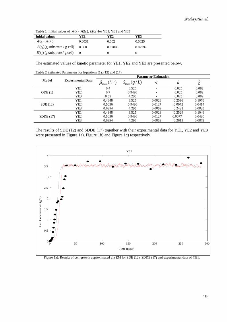
The results of SDE (12) and SDDE (17) together with their experimental data for YE1, YE2 and YE3
were presented in Figure 1a), Figure 1b) and Figure 1c) respectively.
Figure 1a): Results of cell growth approximated via EM for SDE (12), SDDE (17) and experimental data of YE1.
0 50 100 150 200 250 300 0
0.5
1
1.5
2
2.5
3
3.5
4
Time (Hour)
Cel
l C
on
centr
atio
n (
g/L
)
YE1
Jurnal KALAM Vol. 4, No. 1, Page 13 - 25
20
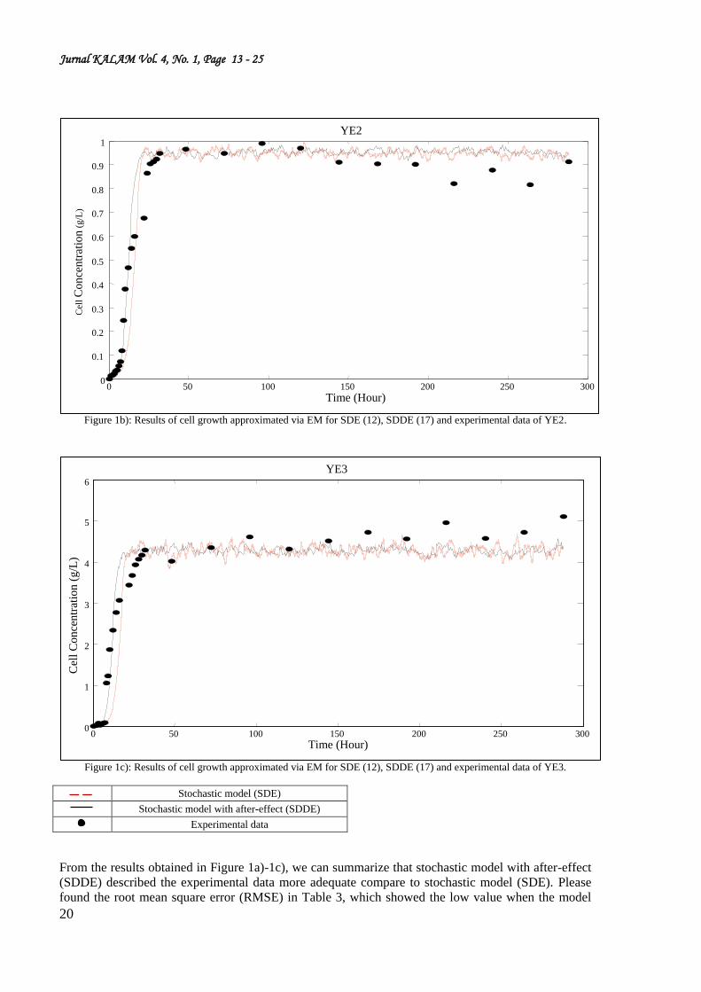
Figure 1b): Results of cell growth approximated via EM for SDE (12), SDDE (17) and experimental data of YE2.
Figure 1c): Results of cell growth approximated via EM for SDE (12), SDDE (17) and experimental data of YE3.
Stochastic model (SDE)
Stochastic model with after-effect (SDDE)
Experimental data
From the results obtained in Figure 1a)-1c), we can summarize that stochastic model with after-effect
(SDDE) described the experimental data more adequate compare to stochastic model (SDE). Please
found the root mean square error (RMSE) in Table 3, which showed the low value when the model
0 50 100 150 200 250 300 0
1
2
3
4
5
6
Time (Hour)
Cel
l C
on
cen
trat
ion
(g
/L)
YE3
0 50 100 150 200 250 300 0
0.1
0.2
0.3
0.4
0.5
0.6
0.7
0.8
0.9
1
Time (Hour)
Cel
l C
on
cen
trat
ion
(g/L
)
YE2
Norhayatiet. al.
21
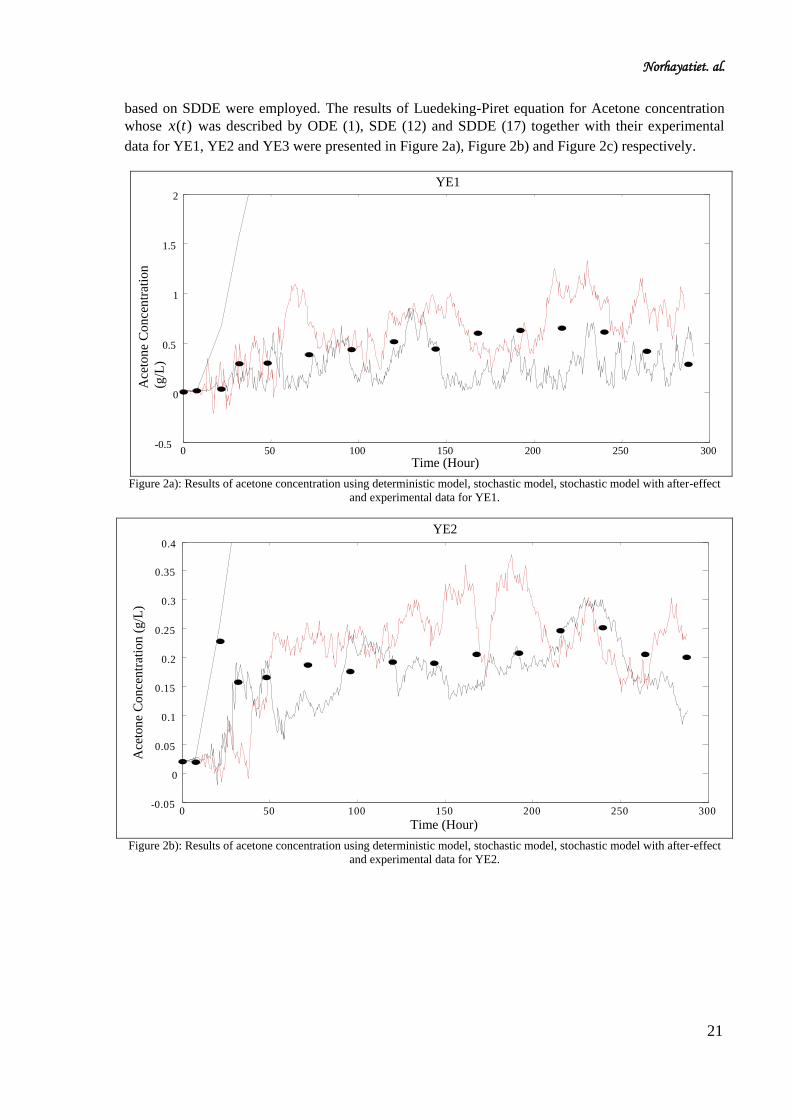
based on SDDE were employed. The results of Luedeking-Piret equation for Acetone concentration
whose )(tx was described by ODE (1), SDE (12) and SDDE (17) together with their experimental
data for YE1, YE2 and YE3 were presented in Figure 2a), Figure 2b) and Figure 2c) respectively.
Figure 2a): Results of acetone concentration using deterministic model, stochastic model, stochastic model with after-effect
and experimental data for YE1.
Figure 2b): Results of acetone concentration using deterministic model, stochastic model, stochastic model with after-effect
and experimental data for YE2.
0 50 100 150 200 250 300 -0.05
0
0.05
0.1
0.15
0.2
0.25
0.3
0.35
0.4
Time (Hour)
Ace
ton
e C
on
cen
trat
ion
(g
/L)
YE2
0 50 100 150 200 250 300 -0.5
0
0.5
1
1.5
2
Time (Hour)
Ace
ton
e C
on
cen
trat
ion
(g/L
)
YE1
Jurnal KALAM Vol. 4, No. 1, Page 13 - 25
22
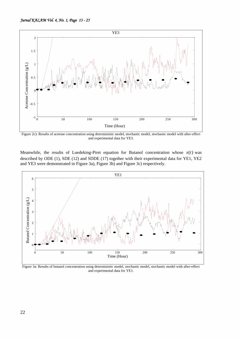
Figure 2c): Results of acetone concentration using deterministic model, stochastic model, stochastic model with after-effect
and experimental data for YE3.
Meanwhile, the results of Luedeking-Piret equation for Butanol concentration whose )(tx was
described by ODE (1), SDE (12) and SDDE (17) together with their experimental data for YE1, YE2
and YE3 were demonstrated in Figure 3a), Figure 3b) and Figure 3c) respectively.
Figure 3a: Results of butanol concentration using deterministic model, stochastic model, stochastic model with after-effect
and experimental data for YE1.
0 50 100 150 200 250 300
0
1
2
3
4
5
6
Time (Hour)
Buta
no
l C
on
cen
trat
ion
(g
/L)
YE1
0 50 100 200 250 300 -1
-0.5
0
0.5
1
1.5
2
150
Time (Hour)
Ace
ton
e C
on
cen
trat
ion
(g
/L)
YE3
Norhayatiet. al.
23
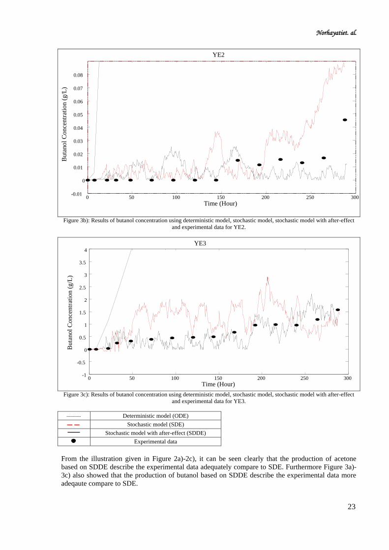
Figure 3b): Results of butanol concentration using deterministic model, stochastic model, stochastic model with after-effect
and experimental data for YE2.
Figure 3c): Results of butanol concentration using deterministic model, stochastic model, stochastic model with after-effect
and experimental data for YE3.
Deterministic model (ODE)
Stochastic model (SDE)
Stochastic model with after-effect (SDDE)
Experimental data
From the illustration given in Figure 2a)-2c), it can be seen clearly that the production of acetone
based on SDDE describe the experimental data adequately compare to SDE. Furthermore Figure 3a)-
3c) also showed that the production of butanol based on SDDE describe the experimental data more
adeqaute compare to SDE.
0 50 100 150 200 250 300 -1
-0.5
0
0.5
1
1.5
2
2.5
3
3.5
4
Time (Hour)
Bu
tano
l C
on
cen
trat
ion
(g
/L)
YE3
0 50 100 150 200 250 300 -0.01
0
0.01
0.02
0.03
0.04
0.05
0.06
0.07
0.08
Time (Hour)
Bu
tano
l C
on
cen
trat
ion
(g
/L)
YE2
Jurnal KALAM Vol. 4, No. 1, Page 13 - 25
24
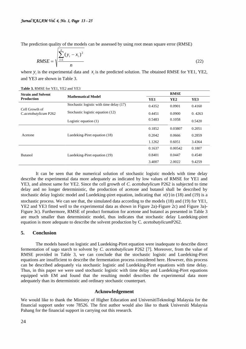
The prediction quality of the models can be assessed by using root mean square error (RMSE)
n
xy
RMSE
n
i
ii
1
2)(
(22)
where iy is the experimental data and ix is the predicted solution. The obtained RMSE for YE1, YE2,
and YE3 are shown in Table 3.
Table 3. RMSE for YE1, YE2 and YE3
Strain and Solvent
Production Mathematical Model
RMSE
YE1 YE2 YE3
Cell Growth of
C.acetobutylicum P262
Stochastic logistic with time delay (17)
0.4352 0.0901 0.4160
Stochastic logistic equation (12)
0.4451 0.0900 0. 4263
Logistic equation (1) 0.5483
0.1058
0.5420
Acetone Luedeking-Piret equation (18)
0.1852 0.03807 0.2051
0.2042 0.0666 0.2859
1.1262 0.6051 3.4364
Butanol Luedeking-Piret equation (19)
0.1637 0.00542 0.1807
0.8401 0.0447 0.4540
3.4007 2.0022 9.4259
It can be seen that the numerical solution of stochastic logistic models with time delay
describe the experimental data more adequately as indicated by low values of RMSE for YE1 and
YE3, and almost same for YE2. Since the cell growth of C. acetobutylicum P262 is subjected to time
delay and no longer deterministic, the production of acetone and butanol shall be described by
stochastic delay logistic model and Luedeking-piret equation, indicating that )(tx in (18) and (19) is a
stochastic process. We can see that, the simulated data according to the models (18) and (19) for YE1,
YE2 and YE3 fitted well to the experimental data as shown in Figure 2a)-Figure 2c) and Figure 3a)-
Figure 3c). Furthermore, RMSE of product formation for acetone and butanol as presented in Table 3
are much smaller than deterministic model, thus indicates that stochastic delay Luedeking-piret
equation is more adequate to describe the solvent production by C. acetobutylicumP262.
5. Conclusion
The models based on logistic and Luedeking-Piret equation were inadequate to describe direct
fermentation of sago starch to solvent by C. acetobutylicum P262 [7]. Moreover, from the value of
RMSE provided in Table 3, we can conclude that the stochastic logistic and Luedeking-Piret
equations are insufficient to describe the fermentation process considered here. However, this process
can be described adequately via stochastic logistic and Luedeking-Piret equations with time delay.
Thus, in this paper we were used stochastic logistic with time delay and Luedeking-Piret equations
equipped with EM and found that the resulting model describes the experimental data more
adequately than its deterministic and ordinary stochastic counterpart.
Acknowledgement
We would like to thank the Ministry of Higher Education and UniversitiTeknologi Malaysia for the
financial support under vote 78526. The first author would also like to thank Universiti Malaysia
Pahang for the financial support in carrying out this research.
Norhayatiet. al.
25
References
[1] Arifah B. (2005). Applications of Stochastic Differential Equations and Stochastic Delay Differential Equations in
Population Dynamics. PhD Thesis, University of Strathclyde.
[2] Bailey, J. E. & Ollis, F. D. (1986). Biochemical Engineering Fundamentals, 2nd Edition, McGraw-Hill.
[3] Baker, C. T. H. and Buckwar, E. (2000). ‘Numerical Analysis of Explicit One-Step Methods for Stochastic Delay
Differential Equations.’London Mathematical Society Journal Comput. Math., 3: 315-335.
[4] Buckwar, E. (2000). ‘Introduction to the numerical analysis of stochastic delay differential equations.’Journal of
Computational and Applied Mathematics, 125: 297-307.
[5] Haliza A. R., Arifah B, Mohd Khairul Bazli, Norhayati R., Madihah M. S. (2009). ‘Nonlinear Parameter
Estimation of Stochastic Differential Equations.’2nd International Conference and Workshops on Basic and
Applied Sciences and Regional Annual Fundamental Science Seminar, 44-48.
[6] Hutchinson, G. E. (1948). ‘Circular causal system in ecology.’Ann. NY Acad. Sci. 50: 221-246.
[7] Hu, Y. Mohammed, S. E. A. and Yan, F. (2004).‘Discrete time approximation of stochastic delay equations: the
Milstein scheme.’Ann. Probab. 32 (1A): 265-314.
[8] Kuchler, U. and Platen, E. (2000). ‘Strong discrete time approximation of stochastic differential equations with
time delay.’Mathematics and Computers in Simulation, 54: 189-205.
[9] Madihah M. S. (2002). Direct Fermentation of Gelatinised Sago Starch to Solvent (Acetone Butanol-Ethanol) by
Clostridium Acetobutylicum P262. PhD Thesis, University Putra Malaysia.
[10] Madihah M.S., Liew S. T. and Arbakariya A. (2008). The Profile of Enzymes Relevant to Solvent Production
during Direct Fermentation of Sago Starch by Clostridium saccharobutylicum P262 Utilizing Different pH Control
Strategies. Biotechnology and Bioprocess Engineering, 13, 33-39.
[11] Mao, X. (2008). Stochastic Differential Equations and Applications, 2nd Edition, Horwood Publishing.
[12] Mohd. KhairulBazli M. A., Arifah B., Madihah M. S. &Haliza A. R. (2009). ‘Stochastic Growth of C.
acetobutylicum,’2nd International Conference and Workshops on Basic and Applied Sciences and Regional Annual
Fundamental Science Seminar, 146-149.
[13] Mohd. KhairulBazli M. A., Stochastic Modeling of The C. Acetobutylicum and Solvent Productions in
Fermentation.’ preprint.
[14] Mohammed, S.E.A. (1984). Stochastic Functional Differential Equations. Pitman Advanced Publishing.
[15] Norhayati R., Arifah B., Yeak S. H., Haliza A. R., Madihah M. S. and MohdKhairulBazli (2009). ‘The
Performance of Euler-Maruyama and 2-stage SRK in Approximating the Strong Solution of Stochastic Model.’2nd
International Conference and Workshops on Basic and Applied Sciences and Regional Annual Fundamental
Science Seminar, 138-141.
[16] Norhayati R., Arifah B., Yeak S. H., Haliza A. R. and Madihah M. S. (2010). ‘The Performance of Euler-
Maruyama, 2-Stage SRK and 4-Stage SRK in Approximating the Strong Solution of Stochastic
Model.’JurnalSainsMalaysiana39(5): 851–857
[17] Norhayati R., Arifah B., Yeak S. H., Haliza A. R., Madihah M. S. and MohdKhairulBazli (2010).‘Stochastic
Model of Gelatinised Sago Starch to Solvent Production by C. acetobutylicum P262.’ Regional Conferences on
Statistical Sciences 2010 (RCSS’10).
[18] Yerushalmi, L., Volesky, B. And Votruba, J. (1986).‘Modelling of culture kinetics and physiological for
Clostridium acetobutylicum.’ Journal of Canadian Chemical Engineering, 64: 607-616.