VOT 74120 DEVELOPMENT OF AN ON-LINE AND … · sektor komersil telah menggunakan 19 peratus...

VOT 74120

DEVELOPMENT OF AN ON-LINE AND INTELLIGENT ENERGY SAVING SCHEME FOR A COMMERCIAL BUILDING

(PEMBINAAN SYSTEM PENJIMAT TENAGA PINTAR SECARA BERTERUSAN UNTUK BANGUNAN KOMERSIL)

Md. Shah Majid

Herlanda Windiarti

Saiful Jamaan

PUSAT PENGURUSAN PENYELIDIKAN UNIVERSITI TEKNOLOGI MALAYSIA

2006

VOT 74120


(PEMBINAAN SYSTEM PENJIMAT TENAGA PINTAR SECARA BERTERUSAN UNTUK BANGUNAN KOMERSIL)

Md. Shah Majid

Herlanda Windiarti

Saiful Jamaan

RESEARCH VOTE NO : 74120

Jabatan Elektrik Kuasa Fakulti Kejuruteraan Elektrik Universiti Teknologi Malaysia

2006

1

Abstrak

Di Malaysia, selama 2 dekad terakhir, permintaan untuk sektor komersil

meningkat pada purata 7.5 peratus pada 1980an dan 7.7 peratus pada 1990an

melebihi 5.9 peratus pertumbuhan GDP dan 7 peratus dari masa yang sama. Saat ini,

sektor komersil telah menggunakan 19 peratus daripada jumlah penggunaan tenaga

untuk semua sektor. Mengikut konteks bangunan komersil, penyaman udara ialah

pengguna tenaga yang utama yang memakai 70 peratus tenaga elektrik sementara 30

peratus digunakan untuk lampu dan beban lainnya. Projek penyelidikan ini ialah

merekabentuk dan membina sistem kawalan penyaman udara dan sistem kawalan

penyusup cahaya luar. Fuzzy akan digunakan untuk menentukan nilai pasti dari

isyarat kawalan yang bertujuan untuk mengenal pasti dan mengawas penggunaan

tenaga secara efisien. Pembinaan skema pintar kawalan tenaga boleh mengawal

penggunaan tenaga bangunan komersil dengan menggunakan pengawas secara

berterusan.

2


Abstract

(Keywords:………….. )

In Malaysia, during the past two decade, demand for commercial sector grew

rapidly, increasing at an average rate of 7.5 percent in the 1980s and 7.7 percent in

1990s, surpassing the GDP growth of 5.9 percent and 7 percent over the

corresponding period. At present, the commercial sector has utilized 19% of the total

energy usage for the all sectors. In the context of commercial building, the air

conditioning is the main energy usage which consumes 70% of the electrical energy

used while the remaining 30% used for lighting and other loads. This research

project is to design and develop an Air Conditioning control system and external

light infiltration control system. Fuzzy will be used to determine the definite value

of control signal in order to identify and to monitor the energy usage in the efficient

way. The development of this proposed energy intelligent control scheme would be

able to control the energy consumption of the commercial building using on-line

monitoring.

Key researchers:

Assoc. Prof. Hj. Md. Shah Majid

Herlanda Windiarti

Saiful Jamaan

Email :

Tel. No : 55 35295

Vote. No : 74120

v


Abstract

(Keywords: Energy saving, Fuzzy, Intelligent)

In Malaysia, during the past two decade, demand for commercial sector grew

rapidly, increasing at an average rate of 7.5 percent in the 1980s and 7.7 percent in

1990s, surpassing the GDP growth of 5.9 percent and 7 percent over the

corresponding period. At present, the commercial sector has utilized 19% of the total

energy usage for the all sectors. In the context of commercial building, the air

conditioning is the main energy usage which consumes 70% of the electrical energy

used while the remaining 30% used for lighting and other loads. This research project

is to design and develop an Air Conditioning control system and external light

infiltration control system. Fuzzy will be used to determine the definite value of

control signal in order to identify and to monitor the energy usage in the efficient

way. The development of this proposed energy intelligent control scheme would be

able to control the energy consumption of the commercial building using on-line

monitoring.

Key researchers:

Assoc. Prof. Hj. Md. Shah Majid

Herlanda Windiarti

Saiful Jamaan

Email :

Tel. No : 55 35295

Vote. No : 74120

vi

CONTENTS

CHAPTER CONTENT PAGE

TITLE i

DEDICATION iii

ABSTRACT v

ABSTRAK vi

CONTENTS vii

LIST OF TABLES x

LIST OF FIGURES xi

LIST OF SYMBOLS xiii

CHAPTER 1 INTRODUCTION

1.1 Introduction 1

1.2 Objective 3

1.3 Scope of Research 3

1.4 Outline Of The Project 3

vii

CHAPTER 2 LITERATURE

2.1 An HVAC Fuzzy Logic Zone Control System and Performance

Results 5

2.2 A Fuzzy Control System Based on the Human Sensation of

Thermal Comfort 16

2.3 A New Fuzzy-based Supervisory Control Concept for The

Demand-responsive Optimization of HVAC Control Systems 31

2.4 Application of Fuzzy Control in Naturally Ventilated Buildings

for Summer Conditions 45

2.5 Thermal and Daylighting Performance of An Automated

Venetian Blind and Lighting System in A Full-Scale Private

Office 62

CHAPTER 3 METHODOLOGY

3.1 Methodology 83

3.2 Programmable Thermostat 94

3.2.1 Testing procedures 94

3.2.2 Operation of the Designed Programmable Thermostat 97

3.3 Software Development 100

3.3.1 Introduction to Borland Delphi 100

3.3.2 Borland Delphi 4 100

3.3.3 Object Pascal and Object Oriented Programming 101

3.3.4 Delphi 4 Development Environment 101

3.3.5 Coding Development 106

viii

CHAPTER 4 RESULT AND DISCUSSION

4.1 Introduction 109

4.2 Tinted Glass, No Blind, All Lamps On 110

4.3 Tinted Glass, No Blind, All Lamps Off 112

4.4 Tinted Glass, With Blind, All Lamps On 114

4.5 Tinted Glass, With Blind, All Lamps Off 116

4.6 Tinted glass,no blind,all lamps On, AC On 118

CHAPTER 5 CONCLUSION AND RECOMMENDATIONS

5.1 Conclusion. 120

5.2 Recommendations 121

REFERENCE

APPENDIX

ix

LIST OF TABLES

TABLE TITLE PAGE

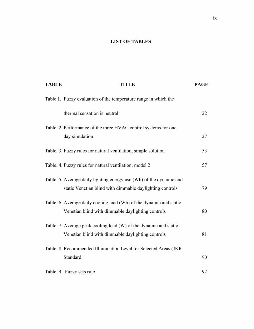
Table 1. Fuzzy evaluation of the temperature range in which the

thermal sensation is neutral 22

Table. 2. Performance of the three HVAC control systems for one

day simulation 27

Table. 3. Fuzzy rules for natural ventilation, simple solution 53

Table. 4. Fuzzy rules for natural ventilation, model 2 57

Table. 5. Average daily lighting energy use (Wh) of the dynamic and

static Venetian blind with dimmable daylighting controls 79

Table. 6. Average daily cooling load (Wh) of the dynamic and static

Venetian blind with dimmable daylighting controls 80

Table. 7. Average peak cooling load (W) of the dynamic and static

Venetian blind with dimmable daylighting controls 81

Table. 8. Recommended Illumination Level for Selected Areas (JKR

Standard 90

Table. 9. Fuzzy sets rule 92

x

LIST OF FIGURES

FIGURE TITLE PAGE

Figure. 1. Fuzzy Logic Controller with MIMO Controller Broken

Into Several SISO Type Controllers. 8

Figure. 4. Temperatures for Zones 1,2, and 3. 12 12

Figure. 5. Zone1, Zone3, and Zone4 heat_flgs. 13

Figure. 6. On/Off cycling of heater for zones 1, 3 and 4. 13

Figure. 7. Zone1-bottom graph, Zone3-top graph, Zone4-middle

graph 14

Figure. 8. Maximum and Minimum Temperature 14

Figure. 9. Zone Temperatures 15

Figure. 10. Zone Heat Flags 15

Figure. 11. PMV and thermal sensation 19

Figure 12. TCL-based Control of HVAC system 20

Figure. 13. TCL-based fuzzy sytem 21

Figure. 14. Membership functions used in the personal-dependant

fuzzy subsystem 23

Figure. 15. Membership functions used to evaluate the optimal air

temperature setpoint 25

Figure. 16. Outdoor temperature and heat gains 28

xi

Figure. 17. The personal-dependant parameters profiles during

simulation (for 1 day) 28

Figure. 18. Simulation results of the HVAC control system based on

comfort level for heating mode 29

Figure.19. Simulation results of the HVAC control system based on

night setback technique 30

Figure. 20. Simulation results of the HVAC control system with

constant thermostat setpoint 30

Figure. 21. The fuzzy based supervisory control and monitoring

system for indoor temperature and sir exchange rate is

superimposed to the temperature and ventilation control

loops 33

Figure. 22. Heuristic membership functions µcomf in dependence of

the perception temperature Top (a), the relative humidity

φ(b) and tbe CO2 – concentration (c). Dotted lines are the

membership functions based on binary logic 39

Figure. 23. Dependence of the optimal indoor temperature TºI,ref and

the air exchange reference AERºref on the slider position λ

and the outdoor temperature To 40

Figure. 24. Simulation at slider positions ,,max economy” (λ = 0.01),

,,medium” (λ = 0.5) and ,,max comfort” (λ = 0.99) 44

Figure. 25. The location of the sensors inside the test room and

across the louver 47

Figure.26. Basic Configuration of Fuzzy Logic Controller 50

xii

Figure.27. Membership functions for inside temperature 50

Figure. 28. Membership functions for outside temperature 51

Figure. 29. Membership function describing wind velocity. 51

Figure. 30. Membership function describing rain 52

Figure. 31. Membership functions for linguistic variables describing

opening position 53

Figure. 32. Outside temperature and the corresponding five

membership functions 54

Figure. 33. Louver opening and the corresponding four membership

functions 55

Figure. 34. The outside conditions for the test on 19 and 22 June 57

Figure. 35. The temperature variations with height at all four

locations 59

Figure. 36. Simulated louver opening for the test 1 outside

conditions and different inside temperatures 59

Figure. 37. Simulated louver opening for the test 2 outside

conditions and different inside temperatures 60

Figure. 38. Simulated louver opening for the case of fuzzy control

model 2 (Table 2) 60

Figure.39. Simulated louver opening for the case of input data

recorded during test 1 61

Figure. 40. Floor plan and section view of full-scale test room 67

xiii

Figure. 41. Site plan (Oakland, CA) 68

Figure. 42. Interior view of testbed 69

Figure. 43. View of surrounding outside the testbed window 69

Figure. 44. Schematic of automated Venetian blind/lighting system 71

Figure. 45. Daily lighting load (kWh) of the base case and prototype

venetian blind/lighting systems, where the base case was

defined by three static blind angles, 0º (horizontal), 15º,

and 45º. Diagonal lines on the graph show percentage

differences between the base case and prototype. Both

cases were defined by the prototype continuous dimming

lighting control system or, within a limited set of tests,

the lighting control systems with no dimming controls

(‘no dayltg’). Lighting power density is 14.53 W/ft2),

glazing area is 7.5 m2 (80.8 ft2), and floor area is 16.96

m2 (182.55 ft2). Data were collected from June 1996 to

August 1997. Measurement error between test room is 12

± 46 Wh (2.6 ± 5.4%). 75

Figure. 46. Daily cooling load (kWh) of the base and prototype

Venetian blind/lighting systems, where the base case

defined by three static blind angles, 0º (horizontal), 15º,

and 45º. Measurement error between rooms for loads

greater than 5 kWh was 87 ± 507 Wh (0.5 ± 5%), and for

loads within 1.5 – 5 kWh was 534 ± 475 Wh (15 ± 12%).

Diagonal lines on the graph show percentage differences

between the base case and prototype. Both cases were

defined by the prototype continuous dimming lighting

control system or, within a limited set of tests, the

lighting control systems with no dimming controls (‘no

xiv

dayltg’). Lighting power density is 14.53 W/m2 (1.35

W/ft2), glazing area is 7.5 m2 (80.8 ft2), and floor area is

16.96 m2 (182.55 ft2). Data were collected from June

1996 to August 1997. 77

Figure. 47. Peak cooling load (W) of the base case and prototype

Venetian blind/lighting systems, where the base case was

defined by three static blind angles, 0º, 15º, and 45º.

Measurement error between room was -24 ± 114 W (-0.6

± 6.4%). Diagonal lines on the graph show percentage

differences between the base case and prototype. Both

cases were defined with the prototype continuous

dimming lighting control system, or within a limited set

of tests, with no dimming controls (‘no dayltg’). Lighting

power density is 14.53W/m2 (1.35 W/ft2), glazing area is

7.5 m2 (80.8 ft2), and floor area is 16.96 m2 (182.55 ft2).

Data were collected between June 1996 and August 1997 78

Figure.48a. The furnace is the part of the split-system residential air

conditioner inside the room 85

Figure.48b. The condenser unit is part of a split-system residential

air conditioner and is outside the room 85

Figure 49. A wiring diagram for a split-system air-conditioning unit

with the evaporator fan in the furnace, and the

compressor and condenser fan in the condensing unit

outside the house 87

Figure 50. Ladder diagram for split-system air-conditioning unit 87

Figure. 51. Diagram block of fuzzification function 91

xv

Figure. 52. Block Diagram of an On-line and Intelligent Energy

Saving Scheme for a Commercial Building 93

Figure. 53. Simple LED Driving Circuit Diagram 95

Figure. 54. Simple LED Driving Circuit 95

Figure.55. Programmable Thermostat Diagram 96

Figure. 56. Programmable Thermostat 97

Figure. 57. Project Flow Chart 99

Figure. 58. Delphi IDE 102

xvi

LIST OF SYMBOL

PSC - Single Phase Compressor

ASHRAE - American Society of Heating, Refrigerating and Air

conditioning Engineers

PMV Predicted Mean Vote

ADC Analog to Digital Converter

LED Light Emitting Diode

VCL Visual Component Library

OOP Object Oriented Programming

° Degree

Ω Ohm

1

CHAPTER I

INTRODUCTION

1.1 Introduction

“An On-line and Intelligent Energy Saving Scheme” can provide alternative

options in developing strategies that contribute to the optional use of resources.

Considerable improvement can be achieved in commercial sector. Further reduction in

total energy consumption can be made possible by better load management and control.

Air Conditioning (AC) System consume more than 70% of the electrical energy

used in P07 building Faculty of Electrical Engineering and 30% used for lighting and

other power consumption according to the online monitoring record[1].

In human life, human always try to adapt with environment. It is shown that

people always try to have a comfortable environment. It can be seen on the progress of

planning design for activity places.

With air conditioning, it can be up grading human life into a better life in order

to improve performance by giving a comfort place to conduct activities.

2

Average of human skin surface temperature in a tropical zone is 33°C [2]. This

condition will be achieved if heat radiation is equal to heat produce. People would not

suddenly feel the coldness if temperature is being changed in neutral band which is

± 1.5°C.

Because of that human body will react quickly if temperature is changing

suddenly which caused blood stream become smaller, then the differences of outdoor

temperature and indoor cooling temperature is preferable not further than 7°C [2].

In order to obtain temperature differences using temperature cooling setting

which is from outdoor temperature changing and indoor activity, then it is necessary to

control Air Conditioning Systems continuously.

In Universiti Teknologi Malaysia (UTM) especially FKE almost in every

building is fully equip with Central Air Conditioning which type is “Water Cooled

Packages Units” which is fully equip with Water Cooling Systems from Cooling Tower

to every AHU and also fully equip with Split Air Conditioning.

Existed temperature control using conventional thermostat or manual thermostat

is located in every split AC and AHU room. Thus this gives a different temperature

control value from the set value which has been arranged because of outdoor

temperature influence and air flow which always change and also because of conducted

activity. That is why indoor temperature is lower than thermostat setting. To overcome

this, it is necessary to control the AC continuously in order to achieve the comfort

level. In this research, a control system which control a split AC in the FKE building;

i.e. P07 3rd floor which in this case is “Bilik Mesyuarat Makmal Sistem Tenaga” will

be developed by using Fuzzy Programmable Thermostat in order to improve AC

performance and saving energy.

3

1.2 Objective

i) To design a fuzzy split air conditioning control system.

ii) To design an automated horizontal blind control in synchronization with lighting

system.

iii) To identify the potential of energy saving.

1.3 Scope of Research

The scope of this research work is to develop an On-line and energy saving scheme

for a commercial building. The work focuses on designing the control system for the

room air conditioning system and lighting system using Fuzzy Logic Controller. The

meeting room, Energy System Lab at P07, Faculty of Electrical Engineering will be

used as a model where the research work will take place.

1.4 Outline Of The Project

Chapter Two is the literature review of the research. This chapter provides a

review of some of the research that has been done which is related to this research.

Chapter Three explains the research methodology in this research.

The steps of research methodology are following :

Selection of a model room

On-line data capture

Optimization of conflicting parameters

Design of hardware

On-line implementation

Testing and validation

Costing Analysis

4

Chapter Four is the result and discussion of the project.

Chapter Five is the conclusion of the project and suggestion for further work of the

project.

5

CHAPTER II

LITERATURE REVIEW

Many research works have been done on designing the controller for air

conditioning and the lighting system. The designs, which have different capability in

improving the use of air conditioning, are presented by the researchers in the journal

paper. Among the papers which are related to these works are as follows:

2.1 An HVAC Fuzzy Logic Zone Control System and Performance Results

[6]

Robert N. Lea, Edgar Dohman, Wayne Prebilsky, Yashvant Jani, outline of

the conceptual design of a heating, ventilation, and air conditioning control system

based on fuzzy logic principals is given. This system has been embedded in

microprocessors with interfaces to the sensors, compressor, and air circulation fan

and installed in a test building for performance evaluation. Over the last few years,

several fuzzy logic controllers for temperature control [1, 2, 3, 4, 5, 6, 7] have been

developed and reported in the literature. The first two references provide the details

for temperature control in a heating, ventilation, and air conditioning (HVAC)

system, developed by Togai InfraLogic and Mitsubishi in late 1989 and 1990. This

system was designed to control temperature in commercial buildings and was

reported to achieve a high comfort level with energy savings up to twenty-five

percent. Fuzzy logic temperature control in non-HVAC systems has also shown to be

very effective [5, 6] in simulation environments with a very complicated models of

6

the plant. However, these controllers did not investigate the energy savings for the

overall operations. Their goal was specifically to achieve higher performance from

the given plant.

In reference 7, a fuzzy temperature controller that can adapt to the customer

requirements has been developed for a residential home heating system. The

controller was first developed in a simulation environment and then was

implemented using a micro controller board. Control of the temperature is reasonably

good and is shown to use less energy for the overall operation.

Another thermal control system based on fuzzy logic principals has been

designed, implemented, tested and flown in a Space Shuttle flight in August, 1992

[8]. The system, referred to as the Thermal Enclosure System (TES) and Commercial

Refrigerator/Incubator Module (CRIM) was developed by Space Industries, Inc.,

League City, Texas, and was used in control of temperature in protein crystal growth

experiments on mid-deck Shuttle payloads. Commercially available off-the-shelf

conventional control systems could not maintain the accuracy of +/-0.1 deg C over a

0-40 deg C range that the experiments required. The fuzzy logic controller, however,

was able to control it well.

The fuzzy controller reported is being developed primarily with residential

applications in mind although it will apply easily to commercial setups as well. The

main emphasis is on the use of zone control, as well as the factoring in of relative

humidity measurements, to maintain comfort level and save on energy usage by

regulating the flow of air to the different zones. In the following paragraphs we will

give a brief overview of the system design and results of testing the system in our

laboratory in League City, Texas.

The fuzzy logic HVAC controller is being developed and tested by Ortech

Engineering Inc. under a NASA/JSC Phase II SBIR contract. It has a functional flow

diagram as shown in figure 1. This flow diagram differs from the conventional

systems typically implemented in residential units. Typical conventional temperature

control systems are based on a single input of temperature and a single output which

controls the on/off state of the compressor and fan simultaneously. These types are

known as SISO controllers and they do not take into account the comfort level to

7

address in this project. It should be noted that the functional flow shown in figure 1 is

not just another presentation of a multi-input multi-output (MIMO) controller broken

into several SISO type controllers. It rather takes into account the comfort level via

the measurement of relative humidity and generates an intermediate value of desired

temperature. It also takes into account the effects of overall air circulation in the

house. The main idea is to maintain an acceptable comfort level in the various areas

of the house as needed rather than assumes a homogeneous environment and turns

the compressor on and off based on the reading of one temperature sensor, as is the

usual case.

Three sets of sensor inputs are available to the controller for each zone;

relative humidity, temperature. And zone temperature set point. The testing facility

consists of a variable speed compressor and fan as well as a fixed capacity-heating

element installed in a six-room mobile home. Temperature and relative humidity

from each zone are available on a continuous basis to the control system. The

temperature set points for each zone can be programmed manually or can assume

default values. Outputs of the controller are compressor speed, fan speed, and

heat/cool/off (H/C/OFF) mode. In addition the system outputs vent positions for each

zone to regulate the flow of air for comfort and energy efficiency. These input and

output parameters have been given reasonable ranges, which determine the universe

of discourse for the definition of the fuzzy membership functions.

Relative humidity, R_H, is quantified according to memberships in the fuzzy

sets low, medium, and high, figure 2.a, which are input to the rule base in figure 2.b.

This rule base has the function of computing an adjusted temperature setting based

on the humidity in the facility. The underlying reason for the rule base is to exploit

the fact that when humidity is low, people are comfortable at higher temperatures, as

long as there is adequate air circulation, than they are when the humidity is high.

Membership functions of low, medium, and high are assigned to the output of this

rule base, desired temperature (D_Tmp), figure 2.c. D_Tmp is an internal variable

which has an actual output range of approximately 23-26ºC, which is within the

ASHRAE published comfort range[9] of 22-26ºC.

8

Figure. 1. Fuzzy Logic Controller with MIMO Controller Broken Into Several

SISO Type Controllers.

The defuzzified value of D_Tmp and the actual sensed temperature are used

to compute an internal variable, Error = Temp – D_Tmp. The membership of Error in

N (negative), Z (zero), and P (positive) are computed according to the membership

functions in figure 3.a. Fifure 3.b shows the Compressor Speed Rule Base which has

temperature error as an input as well as relative humidity, R_H. From this rule base a

fuzzy set denoting compressor speed is computed, and defuzzified using the

membership functions in figure 3.c, to give the required speed level of the

compressor in percent of maximum speed.

Figure 2.a

Desired Temperature

Rule Base

Compressor Speed Rule Base

Fan Speed Rule Base

Mode Computation

Comp. Speed

Relative Humidity(I)

Temperature (I) Set Points(I)

Fan Speed Mode H/C/OFF Vent Position (I)

Vent Position Rule Base

Fuzzy Decision Making Rules

9

Figure 2.b

Figure 2.c

Similarly fan speed is computed from a Fan Speed Rule Base and

membership functions for actual sensed temperature and relative humidity R_H.

These membership values and rules are processed to produce a fuzzy set output for

Fan Speed which is then defuzzified to yield a speed in units of percent of maximum

fan speed.

Figure 3.a.

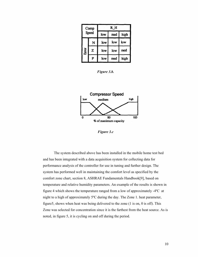
10

Figure 3.b.

Figure 3.c

The system described above has been installed in the mobile home test bed

and has been integrated with a data acquisition system for collecting data for

performance analysis of the controller for use in tuning and further design. The

system has performed well in maintaining the comfort level as specified by the

comfort zone chart, section 8, ASHRAE Fundamentals Handbook[9], based on

temperature and relative humidity parameters. An example of the results is shown in

figure 4 which shows the temperature ranged from a low of approximately -4ºC at

night to a high of approximately 5ºC during the day. The Zone 1. heat parameter,

figure5, shows when heat was being delivered to the zone (1 is on, 0 is off). This

Zone was selected for concentration since it is the farthest from the heat source. As is

noted, in figure 5, it is cycling on and off during the period.

11

Figure 5 also shows the heat flags for zones 3 and 4. Zone 3 heat was off for

the most of the period, while Zone 4 heat was on for a large part of the time which is

consistent with the fact that temperature was lower in Zone 4 than in Zone 3

throughout the period as can be observed in Figure 4.

Figure 6 shows the zones 1,2, and 3 heat flag for two hours on another

afternoon when the outside temperature was in the vicinity of 5ºC. It is seen that the

Zone 1 heat flag is cycling on and off at regular intervals. However, the Zone 3 and

Zone 4 flags came on very short and infrequent intervals. During this period the door

to Zone 1 was open and consequently the warm air from Zone 1 was being dispersed

throughout the zones 3 and 4 which are between Zone 1 and the air return.

Note also in figure 7 that temperature were being maintained in the three

zones at a comfortable level during this period. It may be argued that it is a little

warm in Zone 3, but with the trailer configuration, and with the door to Zone 1 open

as it was during this data period, it is virtually impossible to control Zone 3 and 4

with precision since air from Zone 1 is going to circulate through both zones as it

moves to the return vent.

Figure 8 shows the maximum and minimum temperatures for zones 1, 3 and 4

for still another early morning four hour segment when the outside temperature was

approximately -4ºC. During this period the door to Zone 1 was closed. Figure 9

shows the temperature for each zone during the time period. Figure 10 shows Zone 1

heat cycling on and off at a regular frequency. Also note in figure 9 that zones 3 and

4 temperatures are now maintained at a very good level since with Zone 1’s door

closed they are not so noticeably affected by the air from that zone as they were in

the previous example. This forces Zone 4 to call for heat on a regular basis in order

to maintain its desired temperature as can be seen in figure 10. Zone 3 is still being

heated from Zone 4’s vent as they are fairly close together.

The current system utilizes zone control to regulate the temperature to the

proper comfort level in each of six zones. The current version of the zone control

monitors temperature and humidity and decides a compressor and fan speed setting

for the particular zone. Since we are dealing with a single fan circulation system, we

cannot change fan or compressor speed to a particular zone. Hence we set the

12

compressor and fan speed to a fuzzy set function of the requested speeds of all zones

requiring air flow. Proper flow to the individual zones is controlled through cycling

of the vents from open to closed.

The addition of the zone controller has improved comfort throughout the

trailer. Data collected and analyzed has shown that temperature is held within a

comfortable region in all zones. We have not had time to assess the energy impact,

but expect energy usage to be very efficient. In fact it would be surprising if it is not

better due to the more efficient circulation of the air. It is possible, however, that a

fair comparison will be very difficult to do since, by the nature of a controller

without zone control, we normally have consistent variations in temperature from

room to room which are not controlled. Since we are trying to heat and cool the

house for comfort, we could experience larger energy usage in some cases.

Figure 4. Temperatures for Zones 1,2, and 3

13

Figure 5. Zone1, Zone3, and Zone4 heat_flgs.

Figure 6. On/Off cycling of heater for zones 1, 3 and 4.

14

Figure 7. Zone1-bottom graph, Zone3-top graph, Zone4-middle graph.

Figure 8. Maximum and Minimum Temperature

15

Figure 9. Zone Temperatures

Figure 10. Zone Heat Flags

Later versions of the controller will address the problem of large variations of

the temperature in different zones due to conditions such as occupancy, activity, and

air circulation system configuration. Real savings could result from a modified

version of the zone controller which will add the activity processing from motion

detectors. With this modification the system will not only be able to avoid cooling

one part of the trailer too much, but will also increase the level of required cooling

when the zone is not occupied. It will not turn the system off to an occupied zone,

since relative humidity control will still need to be maintained, but will increase the

16

setpoint for that zone significantly. Similarly, for comfort reasons, if a high activity

level is detected in a zone the setpoint will be lowered since high activity levels lead

to higher relative humidity and increased temperature due to radiation.

Although our laboratory makes use of a variable speed fan compressor, we

are focusing on the more usual situation that occurs in home air conditioners, or even

commercial systems, in which variable speed compressors do not exist due to the

expense. We feel that with a multi-speed circulation fan, with say three speeds, we

could achieve good results in comfort and energy use performance, and as a result

create a system which would be relatively inexpensive to install in a new home or to

retrofit to an existing home. We will also simulate a system with single speed fan to

see if the cost of multi-speed fan installation is justified by increased performance.

Initial results indicate that the system will work well from a comfort level

standpoint. It also seems intuitively clear that by monitoring different zones, and

regulating the air flow into these various zones by shutting off flow to zones where it

is not needed and diverting the air into other zones, will make dramatic differences in

energy use.

It also clear that the system we are building can be easily adapted to a chilled

water system such as may exist in many commercial and state buildings. The logic

would be essentially the same but would require different control devices such as

valves, possibly, for regulating the flow of chilled water, as opposed as to varying the

compressor speed.

2.2 A Fuzzy Control System Based on the Human Sensation of Thermal

Comfort [4]

Maher Hamdi and Gérard Lachiver, Unlike the majority of the existing

residential Heating, Ventilating and Air Conditioning (HVAC) control systems

which are considered as temperature control problems, this paper presents a new

HVAC control technique that is based on the human sensational of thermal comfort.

17

The proposed HVAC control strategy goal is not to maintain a constant indoor air

temperature but a constant indoor thermal comfort. This is realized by the

implementation of a fuzzy reasoning that takes into account the vagueness and the

subjectivity of the human sensation of thermal comfort in the formulation of the

control action that should be applied to the HVAC system in order to bring the

indoor climate into comfort conditions. Simulation results show that the proposed

control strategy makes it possible to maximize both thermal comfort of the occupants

and the energy economy of HVAC systems.

Creating thermal comfort for occupants is a primary purpose of Heating,

Ventilating and Air-Conditioning (HVAC) industry. In this context, there is a

growing interest in the formulation of thermal comfort models that can be used to

control HVAC systems [2, 3, 5, 10]. In spite of these theoretical studies, it is

practically impossible to use the available mathematical models in the design of

HVAC control systems because of three main reasons. First, thermal comfort

calculation requires complex and iterative processing which make it impossible to

implement in real-time applications. Second, the human sensation of thermal comfort

is rather vague and subjective because its evaluation changes according to personal

preferences. Finally, the thermal comfort sensation depends on several variables,

which are difficult to measure with precision and at low cost. The thermal comfort is

a non-linear result of the interaction between four environmental-dependant variables

(air temperature, air velocity, relative humidity, mean radiant temperature) and two

personal-dependant variables (the activity level and the clothing insulation) [2]. To

compute a value of the indoor thermal comfort level, the environmental variables

must be measured at a location adjacent to the occupant and the activity level and the

clothing insulation must be known. In most applications, this is not possible.

To overcome these problems, some studies proposed simplified models of

thermal comfort to avoid the iterative process. Such controllers have been proposed

where simplified thermal sensation indexes have been calculated on the basis of

significant modifications of the original thermal comfort models. Many researchers

carried out that the assumptions under which the simplifications are made are

difficult (or impossible) to reach in residential buildings and they are valid only in

laboratory conditions. Fanger and ISO proposed in [2, 8] to use tables and diagrams

18

to simplify the calculation of the thermal comfort sensation in practical applications.

This method necessitates manual selection of the environmental variable setpoints

that will create optimal indoor thermal comfort. From a practical point of view, this

solution is difficult to use because it requires detailed knowledge of the HVAC

control techniques.

The present paper investigates a new approach to resolve the above-

mentioned problems by using fuzzy modeling. The main advantage of fuzzy logic

controllers as compared to conventional control approaches resides in the fact that no

mathematical modeling is required for the design of the controller. Fuzzy controllers

are designed on the basis of the human knowledge of the system behavior. Since the

human sensation of thermal comfort is vague and subjective, fuzzy logic theory is

well adapted to describe it linguistically depending on the state of the six thermal

comfort dependent variables. In the present work, fuzzy logic is used to evaluate the

indoor thermal comfort level and to indicate how the environmental parameters

should be combined in order to create optimal thermal comfort. The fuzzy rule base

is formulated on the basis of learning Fanger’s thermal comfort model, which is

considered as the most important, and common used one [2].

This paper is organized as follows. First the problem limitation of HVAC

conventional control strategies is exposed. Then, the design of the thermal comfort

fuzzy system is described and applied to the control of the indoor climate of a single

zone building. Finally, the superiority and the effectiveness of the proposed fuzzy

system is verified through computer simulation using MATLAB® and TRNSYS®

algorithms.

Recently, it has been pointed out that controllers that directly regulate

human’s thermal comfort have advantages over the conventional thermostatic

controller [1, 3, 4, 9]. The main advantages are increased comfort and energy

savings. In addition, thermal comfort regulation provides a comfort verification

process. Although mathematical models are available to predict the human sensation

of thermal comfort [2, 5], only the air temperature and the relative humidity are

controlled in the majority of the conventional residential HVAC systems. The

thermal comfort level and the other variables are difficult to quantify and therefore

not used in classic control techniques. Presently, thermal comfort is ensured by the

19

occupants who have to adjust the air temperature setpoint depending on their

perception of the indoor climate. This practice is found to be inadequate to satisfy

occupants desire to feel thermally comfortable. Occupants sitting near sunny

windows or underneath air conditioning ducts or under hot and humid conditions will

find the HVAC control strategy based only on air temperature is not adequate.

Figure. 11. PMV and thermal sensation

Over the past decades, numerous studies of thermal comfort have been

achieved. The widely accepted mathematical representation of thermal comfort is the

predicted mean vote (PMV) index [2]. This index is a real number and comfort

conditions are achieved if the PMV belongs to the [-0.5, 0.5] range [2, 8]. Fig. 1

shows the subjective scale used to describe an occupant’s feeling of warmth or

coolness. However, since the human sensation of thermal comfort is a subjective

evaluation that changes according to personal preferences, the development of a

HVAC control system on the basis of the PMV model had proven to be impossible

[1, 4, 9]. In fact, all classical techniques, including adaptive optimal controllers,

requiring a crisp determination of the comfort conditions, are not suitable for

handling this problem.

20

Figure 12. TCL-based Control of HVAC system

Even if the vagueness and the subjectivity of thermal comfort are the main

obstacles in its implementation in classical HVAC controllers, fuzzy logic is well

suited to evaluate the thermal comfort sensation as a fuzzy concept. The comfort

range can be therefore evaluated as a fuzzy range rather than a crisply defined

comfort zone. Presently, the fuzziness is not eliminated with the conventional HVAC

control techniques, it is simply ignored by these conditions, the HVAC control

system goal is to maintain a desired air temperature in a given indoor space.

However, in everyday life, what is desired is not constant air temperature but

constant comfort conditions. The fuzzy modeling of thermal comfort could be of

importance in the design of such a control system that regulates thermal comfort

level (TLC) rather than temperature levels. The control strategy based on comfort

criteria will regulate the thermal comfort-influencing factors to provide thermal

comfort in the indoor space. The TCL-based fuzzy controller establishes the desired

setpoint values of the environmental variables to be supplied to the HVAC system

and distributed in the building to create a comfortable indoor climate.

Fuzzy

Thermal comfort model

HVAC system

Cold OK Hot

Ta

Tmrt

Vair RH

Icl MADu

Indoor space

The occupant perception of the indoor climate

21

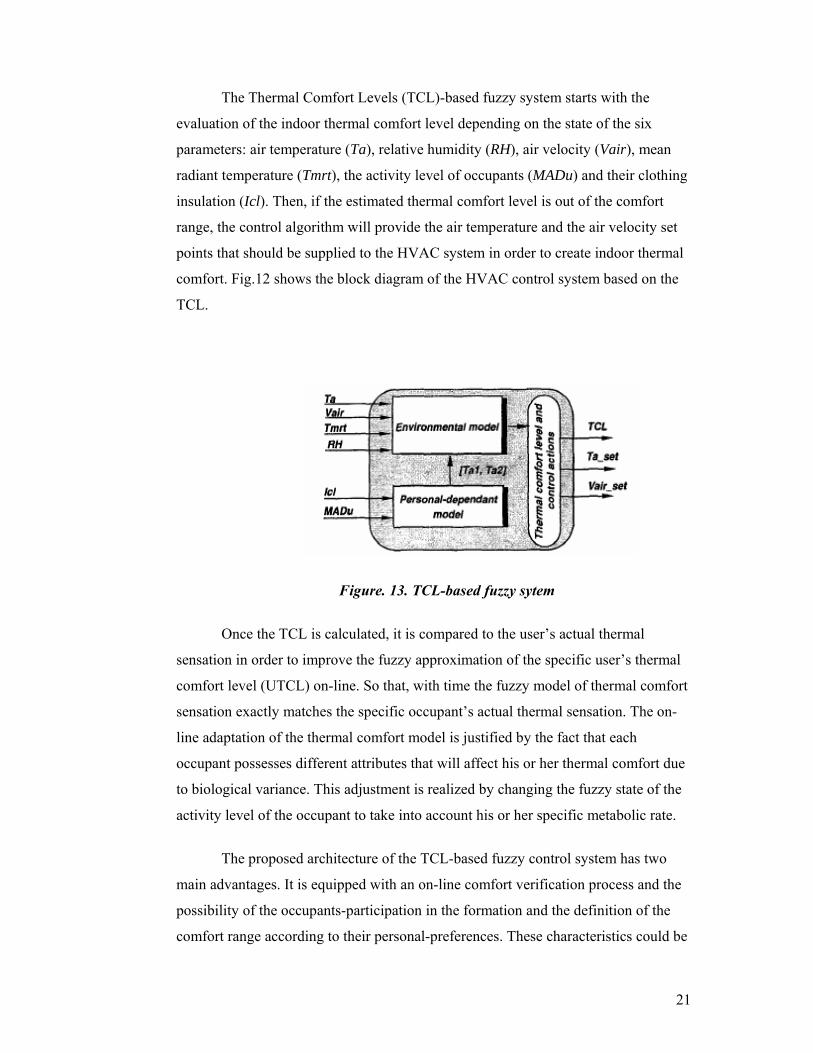
The Thermal Comfort Levels (TCL)-based fuzzy system starts with the

evaluation of the indoor thermal comfort level depending on the state of the six

parameters: air temperature (Ta), relative humidity (RH), air velocity (Vair), mean

radiant temperature (Tmrt), the activity level of occupants (MADu) and their clothing

insulation (Icl). Then, if the estimated thermal comfort level is out of the comfort

range, the control algorithm will provide the air temperature and the air velocity set

points that should be supplied to the HVAC system in order to create indoor thermal

comfort. Fig.12 shows the block diagram of the HVAC control system based on the

TCL.

Figure. 13. TCL-based fuzzy sytem

Once the TCL is calculated, it is compared to the user’s actual thermal

sensation in order to improve the fuzzy approximation of the specific user’s thermal

comfort level (UTCL) on-line. So that, with time the fuzzy model of thermal comfort

sensation exactly matches the specific occupant’s actual thermal sensation. The on-

line adaptation of the thermal comfort model is justified by the fact that each

occupant possesses different attributes that will affect his or her thermal comfort due

to biological variance. This adjustment is realized by changing the fuzzy state of the

activity level of the occupant to take into account his or her specific metabolic rate.

The proposed architecture of the TCL-based fuzzy control system has two

main advantages. It is equipped with an on-line comfort verification process and the

possibility of the occupants-participation in the formation and the definition of the

comfort range according to their personal-preferences. These characteristics could be

22

of importance in the development of modern HVAC systems by using thermal

comfort sensors to quantify the user’s degree of thermal comfort/discomfort.

The fuzzy thermal comfort system is composed of three main subsystems

which are interconnected as shown in Fig.13. The personal-dependant model is used

to approximate the air temperature range [Ta1, Ta2] around which the users should

be in thermal comfort according to the state of the activity level and the clothing

insulation. This subsystem uses the triangular membership functions given in Fig.14

to describe the input and output variables. The fuzzy rule base shown in table 1

represents the set of fuzzy rules that are activated to evaluate the optimal temperature

range.

Table 1. Fuzzy evaluation of the temperature range in which the thermal sensation

is neutral

The 12 fuzzy rules are expressed such as:

• IF the clothing insulation is Light AND the activity level is Low THEN the

air temperature range should be Very High.

• IF the clothing insulation is Heavy AND the activity level is High THEN the

air temperature range should be Very Low.

etc

23

Figure. 14. Membership functions used in the personal-dependant fuzzy subsystem

Once the air temperature range is evaluated, it is supplied to the

environmental model to determine the air temperature and the air velocity setpoints

that will create indoor thermal comfort. The next subsections describe how to derive

these two parameters for any combination of the four environmental variables.

The air temperature setpoint that will provide indoor thermal comfort is

estimated according to the state of the air velocity, the mean radiant temperature and

the relative humidity. This is realized in two steps. First, the air velocity is used to

evaluate the air temperature setpoint for RH = 50%. Then, the air temperature

setpoint is adjusted to compensate any deviation of the relative humidity from 50%.

To this end, δT/δTmrt and the operative temperature (Ta0), which is the optimal

temperature that will create thermal comfort when RH = 50% and Tmrt=Ta, are

Tmrt=Ta, are estimated by using the membership functions and fuzzy terms

(V1,….,V7), (T1,….,T7) and (∆T1,….∆T7) as shown in Fig.15. The fuzzy rule base

represents the effect of the air velocity and the mean radiant temperature on the

necessary air temperature that should create optimal thermal comfort. For a given air

velocity, if the mean radiant temperature in a room is altered, e.g. due to changed

outdoor conditions, or to crowding, or because lights are turned on, a different air

temperature setpoint is required to maintain the indoor thermal comfort. This

24

statement is transformed into a fuzzy reasoning composed of the following seven

fuzzy rules:

• IF Vair is V1 THEN Ta0 is T1 and (δT/δTmrt) is ∆T1







The first rule can be interpreted as if the air velocity is very low, the operative

temperature is close to Tal and an increase in the mean radiant temperature by 1ºC

must be compensated for by a decrease of the temperature by 1ºC. However, the

required air temperature increases and the δT/δTmrt falls with rising velocity. The

deffuzification process is done using the centre of area method and the air

temperature setpoint is therefore calculated as:

Tset = Ta0 + (Tmrt – Ta0). δT/δTmrt (1)

The air velocity setpoint required to maintain thermal comfort conditions is

evaluated by using the mean air temperature ((Ta + Tmrt)/2) as the input of the fuzzy

subsystem. If the mean air temperature is in the temperature range [Ta1, Ta2], then

the air velocity may vary between 0.1 – 1.5 m/s. The same membership functions of

Fig.15 are used to describe the mean air temperature and the velocity setpoint. The

fuzzy rule base used to evaluate the air velocity setpoint according to the mean air

temperature state is deduced on the basis of analyzing the effect of each of them on

the human sensation of thermal comfort. In all seven fuzzy rules are selected and

expressed as:

• IF the mean air temperature is T1 THEN Vair is V1





25



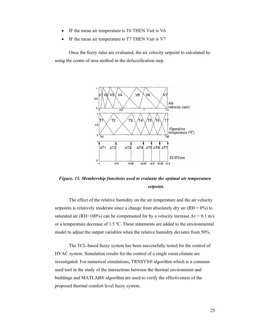
Once the fuzzy rules are evaluated, the air velocity setpoint to calculated by

using the centre of area method in the defuzzification step.

Figure. 15. Membership functions used to evaluate the optimal air temperature

setpoint.

The effect of the relative humidity on the air temperature and the air velocity

setpoints is relatively moderate since a change from absolutely dry air (RH = 0%) to

saturated air (RH=100%) can be compensated for by a velocity increase ∆v = 0.1 m/s

or a temperature decrease of 1.5 ºC. These statements are added to the environmental

model to adjust the output variables when the relative humidity deviates from 50%.

The TCL-based fuzzy system has been successfully tested for the control of

HVAC system. Simulation results for the control of a single room climate are

investigated. For numerical simulations, TRNSYS® algorithm which is a common

used tool in the study of the interactions between the thermal environment and

buildings and MATLAB® algorithm are used to verify the effectiveness of the

proposed thermal comfort level fuzzy system.

26

Fig. 16 shows the outdoor temperature profile ( a January day) and heat gains

that the building was subject to. These included gains due to climatic factors such as

solar gains and to lighting and machines. The profiles of the activity level of the

occupants and their clothing insulation used in the simulation is given in Fig.17.

Fig.18 shows a full day’s simulation result of the TCL-based fuzzy system when

applied for heating mode. It shows the air temperature setpoint in the top graph, the

temperature tracking in the centre and the thermal comfort level in the bottom graph.

These simulation show that the TCL-based fuzzy system is able to adjust the

necessary air temperature setpoint to maintain the indoor thermal comfort as soon as

the personal-dependant variables change.

In order to verify the superiority and the effectiveness of the proposed

thermal comfort fuzzy system, two commonly used conventional techniques are

simulated for the same indoor and outdoor conditions: night setback and constant

setpoint thermostat system. For night setback, the thermostat setpoint was simulated

at 70 F (21.1 C) from 6 a.m. to 10 p.m. and at 60F (15.6 C) from 10 p.m. to 6 a.m

(Fig. 19). On the other side, the thermostat setpoint was simulated at 70F (21.1 C)

for constant setpoint system (Fig. 20). The air temperature tracking and the resulted

thermal comfort level of the occupants versus the hour of the day are given in figures

9 and 10.

For comparison purposes, the performance of the three HVAC control

systems are studied. Table 2 gives the number of hours-per-day in which the

occupants are comfortable (the thermal comfort level is in the [-0.5, 0.5] comfort

range), the energy consumption and the percentage energy savings for each of the

above-studied systems. The heating energy consumption is calculated by the integral

of the simulated system energy demand when operating in the heating mode. Savings

in energy consumption where determined by subtracting the totals obtained with the

TCL fuzzy system and the night setback system from the totals obtained with the

constant setpoint thermostat.

27

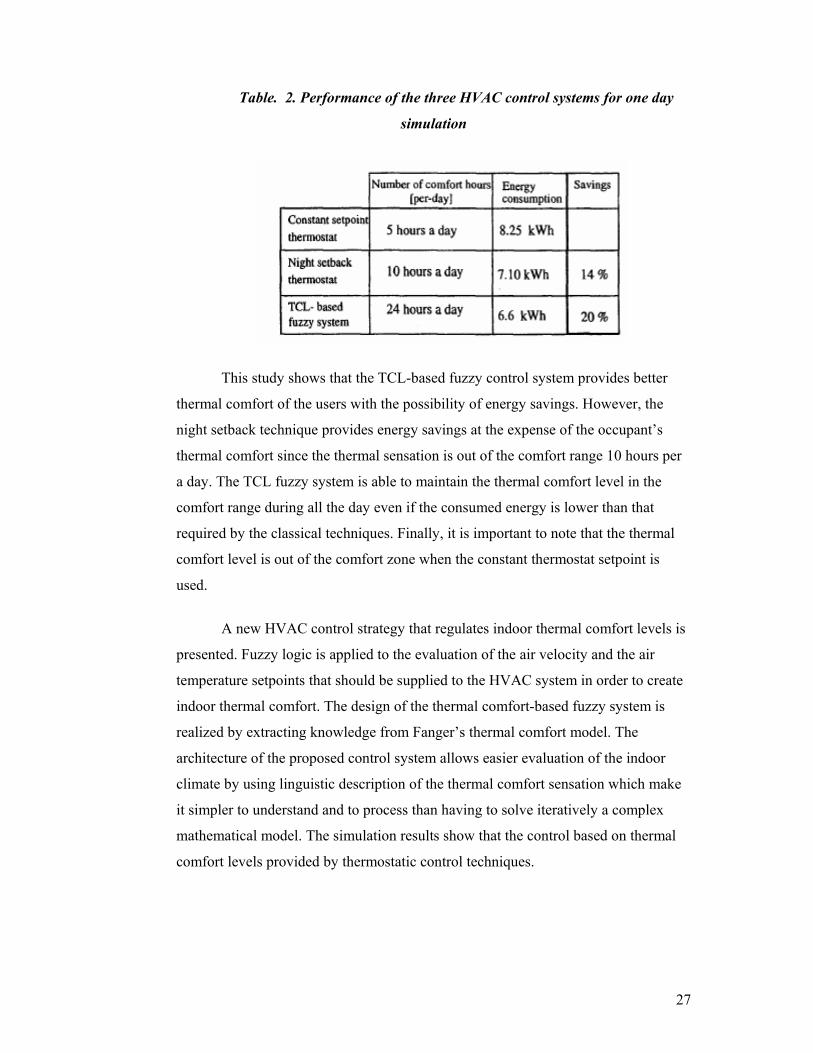
Table. 2. Performance of the three HVAC control systems for one day

simulation

This study shows that the TCL-based fuzzy control system provides better

thermal comfort of the users with the possibility of energy savings. However, the

night setback technique provides energy savings at the expense of the occupant’s

thermal comfort since the thermal sensation is out of the comfort range 10 hours per

a day. The TCL fuzzy system is able to maintain the thermal comfort level in the

comfort range during all the day even if the consumed energy is lower than that

required by the classical techniques. Finally, it is important to note that the thermal

comfort level is out of the comfort zone when the constant thermostat setpoint is

used.

A new HVAC control strategy that regulates indoor thermal comfort levels is

presented. Fuzzy logic is applied to the evaluation of the air velocity and the air

temperature setpoints that should be supplied to the HVAC system in order to create

indoor thermal comfort. The design of the thermal comfort-based fuzzy system is

realized by extracting knowledge from Fanger’s thermal comfort model. The

architecture of the proposed control system allows easier evaluation of the indoor

climate by using linguistic description of the thermal comfort sensation which make

it simpler to understand and to process than having to solve iteratively a complex

mathematical model. The simulation results show that the control based on thermal

comfort levels provided by thermostatic control techniques.

28

Figure. 16. Outdoor temperature and heat gains

Figure.17.The personal-dependant parameters profiles during simulation

(for 1 day)

29

Figure. 18. Simulation results of the HVAC control system based on comfort level

for heating mode.

30

Figure.19. Simulation results of the HVAC control system based on night setback

technique

Figure. 20. Simulation results of the HVAC control system with constant

thermostat setpoint

31

2.3 A New Fuzzy-based Supervisory Control Concept for The Demand-

responsive Optimization of HVAC Control Systems [2]

H.-B. Kuntze and Th. Bernard, In many cases the user of multi-variable

control systems is interested in operating them in a demand or event-responsive

manner according to various, sometimes opposing performance criteria. E.g. within

well isolated low-energy houses there is an increasing requirement to coordinate the

control of heating, ventilation and air conditioning systems (HVAC) in such a way

that both economy and comfort criteria can be considered with a user-specific

tradeoff. In order to find an on-line solution of this multi objective process

optimization problem, a new supervisory control concept has been developed at

IITB. By means of a simple slide button the user is enable to choose his individual

weighting factors for the economy and comfort criteria which are taken to optimize

the reference commands of heating and ventilations of the room occupancy. The

performance of the fuzzy-based multi objective optimization concept, which has

been implemented and is being trialled in a test environment at IITB is analyzed and

discussed by means of practice-relevant simulation results.

Due to the energy crisis and legal energy conservation requirements within

the last decades in construction engineering more and more insulating building

materials and construction techniques have been developed and introduced. By these

measures a remarkably high energy saving has been achieved, however at the cost of

a diminished natural air exchange within the buildings. In order to guarantee a

sufficient air quality and living comfort it is compelling to introduce more and more

controlled ventilation besides controlled heating facilities.

The demand-responsive coordination of both control loops is a tough problem

for untrained users. On the one hand he is free to choose the reference commands of

heating and ventilation control in such a way that his individual cost and comfort

criteria are satisfied. On the other hand the climate state response within the living

room in interaction with the outside climate is very complex and nonlinear. Thus the

user will hardly comprehend all the consequences of his operations with respect to

cost and comfort criteria. Obviously, there is an increasing demand on the HVAC

32

(heating, ventilating and air conditioning) market for a user-friendly integrated

control and monitoring concept of heating and ventilation control systems which is

optimizable with respect to the individual comfort and economy requirements of the

user.

In order to solve the multiobjective on-line optimization problem at the IITB

a new fuzzy-logic supervisory control concept has been developed [1] which can be

applied in principle to comparable problems in different industrial areas.

Interestingly enough fuzzy-based optimization concepts have been almost

exclusively applied to off-line planning and assistance problems in the area of

operations research (cf. e.g. [2]). In the HVAC area fuzzy-logic approaches are

mainly restricted to heating control problems [3].

The fuzzy-based supervisory control concept considered within this paper is

not constrained only to the HVAC applications but can be adapted to various

industrial processes. Especially in the steel and glass industry [4] there is an

increasing demand to control processes optimally in terms of contradictory

performance criteria (e.g. productivity versus product quality).

The climate dynamics within offices and living rooms is more complex as it

seems to be at first sight. Thus, both the comfort perception as well as the energy

consumption depends on the essential climate state variables such as temperature Ti,

relative humidity φi and CO2-concentration CO2i as reference gas of air quality. The

climate state will be disturbed by different measurable or non-measurable influences

of the outside climate as well as of the room occupancy. Measurable disturbance

inputs are e.g. temperature To , relative humidity φo and CO2-concentration CO2o

outside as well as the presence of persons within the room. Non-measurable mainly

stochastic disturbances are the heating flows, water vapor sources, air draft as well as

CO2-emissions caused by present person (cf. fig. 21).

For controlling the room climate in terms of Ti, φ i and CO2i first of all

controllable heating and ventilation facilities have to be installed. However, while the

Ti can be selectively controlled e.g. by radiators φi and the CO2i are strongly coupled

with each other. Thus, the air exchange rate AER which can be controlled by fans or

tilting windows as auxiliary control variable.

33

As regards a feedback-control of Ti as well as φi or CO2, of rooms in the past

different efficient concepts or products have been proposed (cf.e.g. [5]). Much less

considered has been the supervisory control problem of Ti, φi and CO2i.

The supervisory control concept introduced in this paper is based on the

approach that the user chooses the performance requirements in terms of economy

and comfort but not, as usual, the reference values of heating and ventilation

controllers. By means of a simple slide button (“economy-comfort slider”) he/she is

enable to select the weighting factor λ (0<λ<1) of his individual comfort and

economy requirement. If he/she is only interested in minimizing the heating costs

he/she will choose λ → 0. Vice versa he/she will select λ → 1 if he/she prefers a

comfortable living climate. Normally he/she tries to achieve a tradeoff within the

range 0<λ<1.

Figure. 21. The fuzzy based supervisory control and monitoring system for

indoor temperature and sir exchange rate is superimposed to the temperature and

ventilation control loops.

34

Based on the arbitrarily selected cost-comfort weighting, factor λ as well on

the measured inside climate state (Ti, φi, CO2i), outside climate state (To, φo, CO2o)

and the room presence rate (PRES) in the supervisory control system the optimal

reference values of inside temperature control (T*i.ref) and of air exchange rate

AER*ref are computed (cf. fig. 21). The multiobjective optimization of both reference

values is based on a fuzzy-algorithm which will be derived in the following chapter.

In addition to the above nominal operation mode depending on special

daytimes, seasons or events heuristic control elements can be inserted. E.g. in the

absence of persons or during the night time an economy mode can be set

automatically.

A controlled process will be considered in which the state variables x are

completely controllable by the reference values w. Moreover, it will be assumed that

the process will be controlled in terms of two different, sometimes contradictory

performance criteria.

The aim is optimize the reference value w in a balanced way with respect to

both criteria while the user can arbitrarily select his individual weight factor. For

solving this multiobjective optimization problem a concept has been developed

which can be structured into three steps. For better understanding of the following

the optimization of only one reference value wi in terms of two performance criteria

will be considered (cf. box 1).

35

In the first step two performance criteria PC1 and PC2 will be defined by the

fuzzy-membership functions φGK1 and φGK2 which depend only on one state variable.

Since the performance criteria provide a diffused evaluation of process quality which

is especially in climate processes very realistic for solving the multiobjective

optimization problem, the theory of fuzzy decision making [7], [8] can be applied. It

is based on the idea to consider the normalized performance criteria as fuzzy

membership functions which can be optimized by introducing max-min operators.

Physical constraints can be easily considered by setting the membership functions in

the “forbidden” value ranges to zero.

36

In the second step a static or dynamic model is introduced which describes

the relation between state variables x depending on both performance criteria and the

reference value wi to be optimized. Assuming the approximation that the process

behaves quasi-stationarily in the considered optimization interval both performance

criteria can be described in terms of the reference value wi to be optimized.

In the case of strongly nonlinear processes the modeling may sometimes be

difficult. However, for the fuzzy description containing some uncertainty in the

majority of cases it is sufficient to use a simplified physical model in terms of few

significant parameters.

In the third step by using a max-min operation the desired optimal reference

value w*I will be obtained. By introducing the weighting parameter λ the individual

importance of both performance criteria is considered. In the special cases λ → 0 and

λ → 1 only one of both performance criteria PC1 and PC2 is optimized.

The multiobjective optimization approach for one output w*I outlined above

can be easily enlarged to several outputs w* if a weakly coupled MIMO process is

considered of heating and ventilation control loops can be assumed.

For solving the optimization problem in a first step useful performance

criteria of comfort and economy depending on Ti, ref and AERref have to be defined.

Obviously, there are no universal models which can realistically describe the

human comfort perception. In the HVAC technology, however, the limits of comfort

in terms of temperature and air quality are well defined [6]. According to these

standards the perceived temperature Toφ should be within the range 20…22ºC, the

relative humidity φi between 30% and 70% and the CO2-concentration CO2i down to

1000ppm. Since these parameters are only blurred recommendations it is useful to

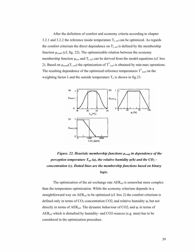
represent them by fuzzy-membership functions e.g. according to fig.22. Obviously,

the shown fuzzy-membership functions µcomf in terms of Top, φi and CO2i represent

the human-like comfort evaluation much better then step – like membership

functions (dotted lines) of the classical binary logic. Moreover, the Fuzzy-parameters

can be easily matched to individual user criteria.

37

The cost of inside temperature and air exchange rate results directly from the

required heating power. Thus, a membership function is required which describes the

economy rate of the HVAC in terms of heating power. A decreasing exponential

function which can be easily parameterized by simple model equations is sufficient

(cf. box 2). In accordance with reality the membership functions show a decrease of

economy in terms of increasing inside temperature and air exchange rate as well as of

decreasing outside temperature.

39

After the definition of comfort and economy criteria according to chapter

3.2.1 and 3.2.2 the reference inside temperature Ti, ref can be optimized. As regards

the comfort criterium the direct dependence on Ti, ref is defined by the membership

function µcomf (cf, fig. 22). The optimmizable relation between the economy

membership function µeco and Ti, ref can be derived from the model-equations (cf. box

2). Based on µcomf(Ti, ref) the optimization of T*i,ref is obtained by min-max operations.

The resulting dependence of the optimized reference temperatures T*I,ref on the

weighting factor λ and the outside temperature To is shown in fig.23.

Figure. 22. Heuristic membership functions µcomf in dependence of the

perception temperature Top (a), the relative humidity φ(b) and tbe CO2 –

concentration (c). Dotted lines are the membership functions based on binary

logic.

The optimization of the air exchange rate AERref is somewhat more complex

than the temperature optimization. While the economy criterium depends in a

straightforward way on AERref to be optimized (cf. box 2) the comfort criterium is

defined only in terms of CO2-concentration CO2i and relative humidity φi but not

directly in terms of AERref. The dynamic behaviour of CO2i and φi in terms of

AERref which is disturbed by humidity- and CO2-sources (e.g. men) has to be

considered in the optimization procedure.

40

Figure. 23. Dependence of the optimal indoor temperature TºI,ref and the air

exchange reference AERºref on the slider position λ and the outdoor temperature

To.

Contrary to the static optimization of Ti, ref in the optimization of AERref the

transition dynamics have to be additionally considered. By means of an internal

predictive model the time response of CO2i and φi is simulated and optimized at each

sampling instant (e.g. every 5 minutes) over a prediction horizon (e.g. 15 minutes) in

terms of the control variables AERref and the initial values of the measured variables

CO2i and φi.

Thus contrary to the feedforward optimization of Ti, ref (cf. chapter 3.2.3) a

dynamic feedback optimization is applied to obtain AER*ref according to the concept

of predictive functional control [9]. The internal model used for the feedback

optimization which describes the dynamics of CO2i and φi in terms of AERref and

internal disturbances, represents a nonlinear differential equation (cf. box 3). By

means of that internal model for a desired dynamic response (e.g. low pass first

order, time constant τ) the comfort membership function µcomf can be described in

terms of AERref.

41

In order to combine µcomf(CO2i) and µcomf (φi) a resulting membership

function can be achieved by applying a min-operator. Finally the optimal value

AER*ref results from a max-min operation of µcomf (AERref) and µeco(AERref).

From the resulting nonlinear function of AER*ref in terms of the weighting

factor λ the strong influence of outside temperature To can be seen (fig. 23). Since the

outside humidity φo depends strongly on To the saturation limit of AER*ref depends

on To as well. Just this dependence demonstrates the advantage of the proposed

supervisory control concept over the non-coordinated operations of a user who

hardly comprehends all the consequences of his heuristic control actions with respect

to economy and comfort. The minimal value AER*i, ref = 0,6/h in the case of highest

42

economy (λ = 0) results from the limit value CO2i ≤1500 ppm recommended for

comfortable air quality in living rooms [6].

In order to investigate system behaviour and performance of the fuzzy-based

supervisory control concept under almost realistic conditions as regards the building

physics or the climate scenario a simulation model has been generated in a

MATLAB/SIMULINK software environment. The physical main structure as well as

the essential influence variables are provided by fig. 21. The conventional ventilation

and heating control loops which are subordinated to the fuzzy control system are

assumed to have PI-behaviour. A sampling interval of ∆t = 6 minutes was chosen.

The considered building physics are characterized by a room volume of V = 50 m3, a

discretization of walls by five layers, an outside wall of a 20 cm brick layer and an

isolation layer of 5 cm (k = 0.54 W/m2k), inside walls of 15 cm brick layers (k = 1.82

W/m2k) as well as one window (k = 2.0 W/m2k). As regards disturbances internal

heating sources Qint = 100 W/Person, a CO2 generating source of CO2dist = 10

Liter/h/person, a water vapour source of xdist = 40g/kg/h/person as well as a constant

temperature of neighbouring rooms Tneuighbour = 15 ºC have been assumed.

From a great manifold of various simulation scenarios one example which

represents the course of a typical winter day assuming three different adjustments of

the fuzzy-based comfort-cost slider is considered in figure. 24. In order to

demonstrate the fuzzy system response with respect to changing room occupancy and

to the corresponding disturbances beginning at 8:00 a.m. the room presence is

successively increased by 1 person per 2 hour cycle. At 6:00 p.m. all five persons

leave the room.

The time response of inside temperature in fig.24 underlines the strong

influence of different adjustments of the comfort-cost slider on the temperature

reference value Toi,ref. It varies within a range which was defined by the chosen

comfort membership function. For the slider positions “max. comfort”, “medium”

and “max. economy” it means Toi,ref = 22 ºC, about 20 ºC and 18 ºC respectively.

Moreover, the influence on the actual room presence PRES can be clearly seen. If the

room is empty the fuzzy-optimization is deactivated, a constant set point Toi,ref = 15

ºC is chosen.

43

From the time response of the air exchange rate AERref an automatic adaption

with respect to altering room occupancy is visible. In the slider position “max.

comfort” the ventilation is activated soon after the presence of the first person in

order to maintain the defined CO2-comfort level of 500 ppm. The strong dependency

between temperature and relative humidity can be seen as well. The cold inflowing

air from outside becomes considerably less humid when heated. Therefore the slider

position “max.comfort” represents a tradeoff between the comfort demand with

respect to CO2-concentration and relative humidity while the CO2-rate increases up

to 700 ppm. Vice versa in the slider position “max. economy” the ventilation is not

activated before the CO2-concentration achieves the defined threshold of 1500 ppm.

Then the relative humidity remains in an uncritical range.

Based on numerous simulations of various realistic scenarios of building

physics and climate it could be proved that a considerable reduction of energy costs

can be achieved by the optimally coordinated fuzzy-supervisory control of heating

and ventilation systems. In the considered case in fig. 24 the required heating energy

of 13.3 kWh at slider position “max comfort” can be reduced by more than 70 % at

3.7 kWh if the slider position “max. economy” is chosen.

In this paper a new fuzzy-based supervisory control concept for HVAC

systems is presented. It enables the untrained user to easily and optimally operate

his/her home heating and ventilation control facilities according to his/her

individually weighted comfort and economy objectives. The performance with

respect to energy saving and comfort improvement is demonstrated by different

realistic simulations. On-going R&D activities deal with the implementation of the

fuzzy concept in a marketable building automation and control system and with the

experimental investigation in a demonstration center at the IITB. The modification of

the fuzzy-based supervisory control concept to completely different multivariable

industrial processes will be the subject of further research.

44

Figure. 24. Simulation at slider positions ,,max economy” (λ = 0.01), ,,medium” (λ

= 0.5) and ,,max comfort” (λ = 0.99).

45

2.4 Application of Fuzzy Control in Naturally Ventilated Buildings for

Summer Conditions [5]

M. M. Eftekhari, L. D. Marjanovic, The objective of this work is to develop

a fuzzy controller for naturally ventilated buildings. Approximate reasoning has

proven to be in many cases more successful control strategy than classically designed

controlled scheme. In this paper the process of designing a supervisory control to

provide thermal comfort and adequate air distribution inside a single-sided naturally

ventilated test room is described. The controller is based on fuzzy logic reasoning

and sets of linguistic rules in forms of IF-THEN rules are used. The inputs to the

controller are the outside wind velocity, direction, outside and inside temperatures.

The output is the position of the opening. A selection of membership functions for

input and output variables are described and analyzed. The control strategy

consisting of the expert rules is then validated using experimental data from a

naturally ventilated test room. The test room is located in a sheltered area and air

flow inside the room, the air pressures and velocities across the openings together

with indoor air temperature and velocity at four locations and six different levels

were measured. Validation of the controller is performed in the test room by

measuring the air distribution and thermal comfort inside the room with no control

action. These data are then compared to the air temperature and velocity with the

controller in action. The initial results are presented here, which shows that the

controller is capable of providing better thermal comfort inside the room.

There is currently a growing worldwide interest in low-energy building

design. An important aspect of this is the goal of maximizing the effectiveness of the

environmental control provided by the building envelope and minimizing the use of

mechanical plant, especially in cooling systems. Much attention has been focused on

taking advantage of natural ventilation; however, as it is driven by forces which are

primarily of an uncertain nature, there is need to control the resulting airflow in order

to maintain comfortable conditions. The ability to effectively control the indoor

environment would considerably enhance the use of natural ventilation in buildings.

46

Current practice in naturally ventilated buildings is mainly manual control of

openings or seasonal operation [1]. The use of negative feedback control for natural

ventilation systems is inhibited by the difficulty of defining a representative sensed

variable. In addition to the feedback loop some rule-based enhancement are required

to take account of particular external conditions.

The principal objective in controlling the thermal environment in occupied

spaces is to minimize the discomfort throughout the occupied region of the space. In

most situations in which conventional feedback control is used, the air is well mixed

and the variation in comfort conditions within the space is relatively small, so the

signal from a single temperature sensor can be used as the controlled variable. In

naturally ventilated spaces the air temperature and speed vary significantly with

position and the form of their distribution also varies with the external conditions and

with the position of the window or other control flow element.

The complexity of the problem suggest that a rule based control system

would be most appropriate. A fuzzy control is particularly suited for controlling

systems that cannot be easily mathematically modeled, but can be described by

experts.

The primary objective of this research was to develop a fuzzy rule based

controller, which can vary the resistance of ventilation opening in order to minimize

the deviation from the desired comfort conditions. Rules were developed based on

performed simulations [2,3] and available expert knowledge. The control strategy

consisting of the expert rules is then validated using experimental data from a

naturally ventilated test room. The test room is located in a sheltered area and air

flow inside the room, the air pressures and velocities across the openings together

with indoor air temperature and velocity at four locations and six different levels

were measured. Validation of the controller is performed in the test room by

measuring the air distribution and thermal comfort inside the room with no control

action. These data are then compared to the air temperature and velocity with the

controller in action. The initial results are presented here, which shows that the

controller is capable of providing better thermal comfort inside the room.

47

Figure. 25. The location of the sensors inside the test room and across the

louvre

An existing portable cabin of light mass is used as a test room for natural

ventilation at Loughborough University, located in a sheltered area. The room is

fitted with four sets of horizontal slats metal louvers, and tracer gas measurements

technique were carried out [4] demonstrated that a minimum ventilation of 8 l/s per

person was achieved inside the test room what corresponds to opening level of 23%

in respect to maximal opening position. To measure the indoor air flow distribution

the room was divided into four zones and for each zone the temperature and velocity

stratification were measured. During summer the internal heat loads inside the room

were three computers, one flow analyzer and two fluorescent luminaries. Due to the

sheltered position of the test room there was no solar gain into the room. During the

experiments the size of the opening at the top and bottom was 0.07 and 0.12m2,

respectively, with a 1.25m distance between the centre of the openings. Details of the

U-values and the thermal capacity of the test room was described fully elsewhere [4].

48

Due to the sheltered nature of the test room, the external environmental

weather conditions local to the test room were measured. Weather station sensors

were mounted locally which measured the wind velocity, direction, outside air

temperature, humidity and pressure. Inside the room mean air velocity and

temperature were measured. The total pressure at top and bottom levels inside and

outside across the louvers was recorded using low-pressure differential transducers.

The reference pressure for all pressure measurements was the static pressure inside

the room taken at approximately 1 m from the floor. Multichannel flow analyzer was

used for the measurements of the inside air temperature and velocity at four locations

and six levels above the floor. The positioning of indoor sensors is shown in Fig. 25.

The linguistic description of the dynamic characteristics of a controlled

process can be interpreted as a fuzzy model of the process. A set of fuzzy control

rules can be derived using experimental knowledge. This approach avoids rigorous

mathematical models and is consequently more robust than a classical approach in

cases which cannot be or are with grate difficulties precisely modeled

mathematically.

The fuzzy logic controller’s goal is to achieve thermal comfort inside the

naturally ventilated room. Based on outside condition and inside temperature (inputs)

the position of the openings (output) will be adjusted. The typical design scheme of

an open loop fuzzy controller [5] which is used is shown in Fig. 26.

The basis of a fuzzy or any fuzzy rule system is the inference engine

responsible for the inputs fuzzification, fuzzy processing and defuzzification of the

output.

In fuzzy control applications to heating and air conditioning systems the usual

number of membership functions describing input variables and actuating signals is

between 3 and 7. Logic behind three membership functions is that in most cases it is

enough to describe quantities or changes as “small”, “moderate” or “big”. In the case

of further expenditure of subsets gets further divided into new three subset (“very

big”, “positive big” and “big” or “very very small”, “very small” and “small”). The

exception can be ambient temperature, which is often described with four

membership functions.

49

Based on comfort criteria and specific aspects of natural ventilation

membership functions for the input and output variables are defined. In Fig.27, the

input variable inside temperature is described in terms of linguistic variables as

“low”, “acceptable” and “high”. Since it is important to establish the relationship

between the inside and outside temperature, the minimum number of linguistic

variables describing outside temperature should be also three. Membership function

describing input variable outside temperature is presented in Fig. 28.

Wind velocity of 7 m/s in natural ventilation applications is marked as a

critical one after which all openings should be closed. Changes in wind speed over a

moderate range does not influence air velocity inside single-sided ventilated space as

much as it does for a cross ventilation. This has been confirmed by performed

measurements and simulation in a test room. This argumentation led to a conclusion

that one membership function describing very strong wind would be enough.

In natural ventilation applications the recording of any rain presence is

compulsory. Opening should be closed or in a safe position in the case of rain

detection as well. Membership functions describing wind velocity and rain presence

are shown in Figs. 29 and 30, respectively.

50

Figure.26. Basic Configuration of Fuzzy Logic Controller

Figure.27. Membership functions for inside temperature.

Knowledge base Rule base

Fuzzification Inference engine Defuzzification

Naturally Ventilated Test Room Crisp inputs Crisp output

fuzzy

input

fuzzy

output

input membership functions

rules table

output membership functions

Outside and inside temp. and Wind vel.

Opening position

51

Figure. 28. Membership functions for outside temperature.

Figure. 29. Membership function describing wind velocity.

52

Control element in the case of natural ventilation only is the opening position.

As any other ventilation control element it should have some predetermined nominal

position which would correlate with min ventilation requirements. In respect to the

nominal position, the area of the openings (output) can increase or decrease, as

presented in Figure.31, allowing more or less air to enter the space depending on

environmental conditions.

Figure. 30. Membership function describing rain.

53

Figure. 31. Membership functions for linguistic variables describing opening

position

Table.3. Fuzzy rules for natural ventilation, simple solution

While the differential equations are the language of conventional control, IF-

THEN rules about how to control the process are the language of fuzzy control.

Fuzzy rules serve to describe the quantitative relationship between variables in

linguistic terms. Instead of developing a mathematical model of a single-sided

natural ventilated space, a different approach has been adopted and knowledge based

system is implemented. The system aims to make the correct decision about how to

move the louvers according to environmental conditions. For summer conditions that

practically means that as long as outside temperature is smaller than inside the

outside air should be let in to allow cooling.

54

Several rule bases of different complexity have been developed for the

controller. One possible set of rules for input variables defined in Figs. 27-30 is given

in Table 3.

The number of rules in the controller will depend on the total number of

linguistic variables. It is certainly possible to describe in more details at least some of

the input variables. In describing outside temperature universe for summer conditions

there is obviously a room for more than three membership functions. Description of

the outside temperature with five membership functions as “very low”, “low”,

“average”, “high” and “very high” is presented in Fig. 32.

Figure. 32. Outside temperature and the corresponding five membership

functions

55

If the outside temperature is described by five membership functions that

allows controller not only to detect the difference between the outside and inside

temperature but also to evaluate its magnitude. In that case it is logical to allow

different levels of louver opening and closure. The louver position described by four

membership functions is presented in Fig. 33. New membership function “closed”, is

introduced in order to make a difference between closure due to security reasons

(rain or wind) and closure due to temperature difference.

For these new membership functions, a new set of IF-THEN rules was

developed, which is given in Table.4.

Figure. 33. Louvre opening and the corresponding four membership functions

56

In this particular case the fuzzifier was very simple; the real input was

fuzzified according to appropriate input membership function [9].

The inference engine applies Mamdani min-max method. A single fuzzy IF-

THEN rule assumes the form

IF x is A and y is B THEN z is C

where A, B and C are fuzzy sets. In IF-THEN rules the term following the IF

statement is called the premise or antecedent and the term following THEN is called

the consequent. Degree to which premise is true is called the degree of applicability

of the premise part usually denoted as β and calculated as t-norm: β = A1 (x1) t B1

(x1). Fuzzy controllers in general have more than one rule. Depending on the input

values some rules are fired and some are not. Each fired rule produces the fuzzy set

output. Overall fuzzy output is obtained by applying the s-norm operator on all rule

outputs: C = C1 s C2 s … s Cn rules. Depending on the definition of t and s norms used

to process fuzzy IF-THEN rules, there are many proposed methods in the literature.

The most common used is direct Mamdani method. In this method the final output

membership function for each output is the union (maximum operator) of the fuzzy

sets assigned to that output after scaling their degree of membership according to

corresponding premise degree of applicability using min operator for t-norm.

The defuzzifier uses the centre of area method to compute the crisp values

needed to drive the actuator:

where Ci(z) are the membership function values of each rule and zj the support values

of the quantization levels.

The weather data for the tests performed on 19 June 1998 (test 1) and 22 June

(test 2) with the wind directly towards the openings (windward) are shown in Fig. 34.

The measured temperatures for all four locations across the room during the test are

shown in Fig. 35. The average inside temperature on all locations during the tests 1

and 2 was 25.6 and 22.34 ºC respectively.

57

Figure. 34. The outside conditions for the test on 19 and 22 June

Table. 4.

58

The control Model 2 was used to test the fuzzy rules shown in Table 2.

Simulation was performed for several different possible levels of inside temperatures

chosen according to Inside Temperature membership functions and for outside

conditions (outside temperature and wind velocity) for both tests. The results for

inside temperature of 19, 21 and 23 ºC for both tests are given in Figs. 36 and 37,

respectively.

For inside temperatures below 19 ºC the opening positions were similar to

that of temperature of 19 ºC as shown in Figs. 36 and 37. In the case of test 1 when

outdoor temperature is considerable “high”, and the inside temperature “low”, the

louvers are open more depending on the wind speed. For the test 2 when outdoor

conditions when outdoor temperature is relatively low, with the further drop outdoor

temperature louvers would be closing down. For temperature higher than 23 ºC the

controller behavior is similar to that of inside temperature of 23 ºC.

59

Figure. 35. The temperature variations with height at all four locations.

Figure. 36. Simulated louver opening for the test 1 outside conditions and different

inside temperatures.

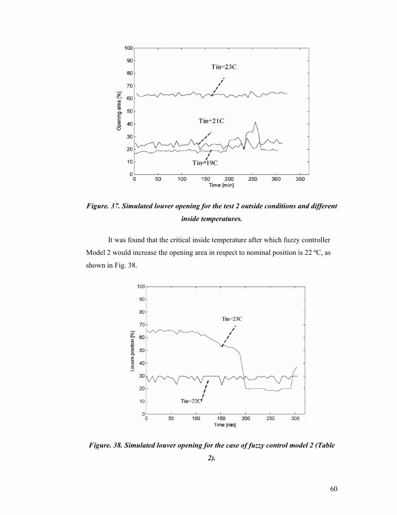
60

Figure. 37. Simulated louver opening for the test 2 outside conditions and different

inside temperatures.

It was found that the critical inside temperature after which fuzzy controller

Model 2 would increase the opening area in respect to nominal position is 22 ºC, as

shown in Fig. 38.

Figure. 38. Simulated louver opening for the case of fuzzy control model 2 (Table

2).

61

On the 19 June no control action upon the position of the louver which was

kept constant (around 23%) resulted in high internal temperature of 25.6 ºC. Based

on weather data recorded during that test and the average inside temperature both

fuzzy control models were compared. The control Model 1 was based on three

membership functions for outside temperature and opening positions. The control

Model 2, used 5 and 4 membership functions for outside temperature and opening

positions respectively. Simulation was performed under MATLAB programming

surrounding and the results are presented in Fig. 39.

Comparing the results for the measured inside temperature of 25.6 ºC, using

both Model 1 and Model 2 controllers, showed that the Model 2 with more

membership functions and therefore larger number of IF-THEN rules, will provide

better control action. Simulation results suggested that a fuzzy controller would

increase opening area with an increase in outside temperature in order to raise inside

temperature levels.

Figure.39.Simulated louver opening for the case of input data recorded

during test 1

62

Two fuzzy control models were developed, using different membership

functions. The results for the measured inside temperature of 25.6 ºC, using both

Model 1 (Table 1) and Model 2 (Table 2) controllers, showed that the Model 2 with

more membership functions and therefore larger number of IF-THEN rules, was

more responsive to the changes in outside conditions. However, the simulation

results indicated that both controllers are capable of responding to the changes in

outside condition by adjusting the opening positions. The opening areas were

decreased once the outside temperature was greater than inside, but control Model 2

resulted in decreasing openings to a minimum level. Such decision appears to be a

better solution, considering that relatively high outdoor temperature levels combined

with too high ventilation rate could lead to higher inside temperatures.

The control Model 2 with more membership functions and therefore larger

number of IF-THEN rules was tested using different inside temperatures and outside

conditions. The results showed that the controller is capable of adjusting the opening

positions with changes in inside and outside conditions.

2.5 Thermal and Daylighting Performance of An Automated Venetian Blind

and Lighting System in A Full-Scale Private Office [1]

E.S. Lee, D.L. DiBartolomeo, S.E. Selkowitz, Dynamic envelop/lighting

systems have the potential to optimize the perimeter zone energy balance between

daylight admission and solar heat gain rejection on a real-time basis, and to increase

occupant comfort. Two side-by-side full-scale offices in Oakland, California were

built to further develop and test this concept. An automated venetian blind was

operated in synchronization with a dimmable electric lighting system to block direct

sun, provide the design workplane illuminance, and maximize view. The research

program encompassed system design refinements, energy measurements, and human

factor tests. In this study, it present lighting energy and cooling load data that were

monitored in this facility over the course of a year. Significant energy savings and

peak demand reductions were attained with this automated venetian blind/lighting

system compared to a static venetian blind with the same dimmable electric lighting

system. Correlations between key weather parameters and cooling end uses under

63

the full range of weather conditions of this sunny, moderate climate. Energy

efficiency estimates were conservative since experience shows that conventional

daylighting control systems and manually operated shading devices are rarely used

effectively in real world applications.

The category of ‘dynamic’ window technologies encompasses numerous

conventional components such as motorized louvers, Venetian blind, and shades, as

well as more advanced glazing systems such as switchable electrochromics,

thermochromics, polymer dispersed liquid crystal glazings, and electrically heated

glazings. These building envelope technologies offer promising energy-efficiency

opportunities and the potential to provide higher quality work environments.

Substantial research has been devoted to passive heating applications, with dynamic

window systems working as heat exchange systems. Computer simulations,

laboratory tests, or reduced-scale field tests document the energy benefits associated

with this application; e.g. automated between-pane Venetian blinds controlled by

temperature and solar position.

For climates with high daylight availability and building types that are

cooling load dominated, dynamic window technologies coupled with daylighting

controls, window technologies that possess a broad range of daylight transmission

and solar heat gain rejection properties can be used to actively optimize daylight,

reduce electric lighting loads, and reduce the respective solar and lighting heat gains

at perimeter zones of commercial buildings. Less research has been devoted to such

systems. While there are dynamic shading or dimmable lighting systems

commercially available today, there are no commercially available today, there are

no commercially available, dynamic window systems that are designed to operate in

synchronization with the lighting system. We have summarized simulation studies

that have been conducted on the electrochromic device coupled with daylighting

controls. Other researchers demonstrated a similar control strategy using external

Venetian blinds and a dimmable electric lighting system in a test cell and a full-scale

occupied building. There are no comprehensive field-monitored performance data

that quantifies the energy benefits of both systems working interactively.

64

In this study, it present results from a full-scale testbed demonstration that

was conducted over the course of a year in two side-by-side, fully furnished but

unoccupied test rooms located in a federal office building. The entire scope of work

included further refinements to a dynamic Venetian blind/lighting system, energy

measurements, and human factors tests. These tests different from earlier reduced-

scale field tests in that the system design was iteratively tuned to solve and

accommodate full-scale, observable issues such as venetian blind behavior, motor

noise, and occupant preferences. The rooms were fully instrumented to collect data

on cooling load, lighting energy consumption, system operation, and environmental

quality. The energy results are documented here.

This research is part of a larger multi-phase research and development

program whose primary objective was to develop integrated building envelope,

daylighting, and lighting systems. The large variation in solar radiation due to

diurnal and seasonal changes of sun and sky conditions is a major cause of both high

energy use and peak demand, and of occupant discomfort. However, there is an

optimum cooling and lighting energy balance between the envelope and lighting

energy balance between the envelope and lighting system that can be used to

advantage to reduce this large variation: daylight can be used to advantage to reduce

this large variation: daylight can be used to offset lighting energy use and the heat

gains associated with the electric lighting system, but the admission of too much

daylight introduces solar heat gains that can increase cooling loads associated with

the window system. By taking an integrated systems approach to combining

disparate components, greater energy savings can be attained with improved

occupant comfort over conventional design practice.

Simulation results from early studies revealed the potential of this concept. In

California, our energy simulation models predicted that 500-800 MW of peak

electricity demand can be saved with this integrated approach over business-as-usual

practice for new construction and partial retrofit of office buildings alone by the year

2005. Since lighting and cooling in commercial buildings constitute the largest

portion of peak electrical demand, promotion of such integrated systems can also

become a cost-effective option for owners and utilities.

65

DOE-2 building energy simulations were used initially to model actively

controlled Venetian blinds with daylighting controls, ‘manually’ operated shading

systems (activated every hour when glare or direct sun was detected), and advanced

electrochromic glazings. Total annual energy savings of 16-26% were attained with

the Venetian blind/lighting system compared to an unshaded low-E spectrally

selective window with daylighting controls in Los Angeles, California. The energy

impact of predictive control algorithms was also investigated in detail.

Field tests using the dual chamber calorimeter Mobile Window Thermal Test

(MoWiTT) facility indicated that the automated Venetian blind/lighting system with

a less than optimal control algorithm was still more than twice as effective at

reducing peak solar gains under clear sky conditions controls, while providing the

same level of useful daylight. A separate year long test was also conducted in a 1:3

reduced-scale test cell to determine the lighting energy savings potential of the

automated Venetian blind/lighting system and to further develop the control

algorithm and hardware solution under real sky conditions. Lighting energy savings

of 37-75% were attained with the dynamic system compared to a partially closed,

static blind with the same lighting control system for south to southwest-facing

windows on clear sunny days.

In terms of evaluating comfort and environmental quality, a RADIANCE

visualization simulation study was conducted to evaluate visual comfort associated

with a dynamic electrochromic glazing. The dynamic window was able to control

the window, interior task, and remote surface luminance levels to within

recommended practice standards over the course of a clear, sunny day in Phoenix,

Arizona. The clear and tinted static glazings were not.

The full-scale test bed facility completed the development process of the

prototype system by enabling us to test and evaluate the design in full-scale. New

energy-efficient technologies must be well tested and proven before they are

introduced to the building industry, to ensure performance and to reduce real and

perceived risk. Through limited tests in actual buildings, performance data can be

provided to industry, utility program managers, or design professionals who need

data to asses the aesthetics, cost and energy performance of the technology. This test

bed demonstration was both R&D facility to help answer research questions and a

66

limited proof-of-concept test, allowing practical ‘bugs’ to be worked out of an

innovative building system.

The full-scale Oakland Federal Building test bed demonstration facility was

designed to measure the electric lighting power consumption and the cooling load

produced by the window and lighting system under realistic weather conditions. The

facility consisted of two side-by-side rooms that were furnished with nearly identical

building materials and furniture to imitate a commercial office-like environment

(Figs. 40-42). Each test room was 3.71 m wide by 4.57 m deep by 2.68 m high

(12.17 ft x 15 ft x 8.81 ft). The southeast-facing windows in each room were

simultaneously exposed to approximately the same interior and exterior

environments between the two rooms could be compared.

Because this facility was installed in an existing commercial office building

and in built-up urban area, a limited number of external conditions was measured. A

datalogging station located on the roof of a five-story adjacent building wing

monitored global and diffuse horizontal exterior illuminance, horizontal global solar

radiation, and outdoor dry bulb temperature (shielded from solar radiation). Interior

measurements included horizontal workplane illuminance, vertical illuminance,

power consumption of all plug loads and mechanical equipment, cooling load,

interior air temperatures, and other information pertaining to the status of the

dynamic window and lighting system.

67

Figure. 40. Floor plan and section view of full-scale test room.

Identical automated Venetian blind/lighting systems were installed in each

room so that the position of the prototype and base case systems could be

interchanged. Both test rooms were located in the southeast corner of a larger

unconditioned, unfinished space (213 m2, 2300 ft2) on the fifth floor of a 18 story

tower. Room A was located to the east of Room B and was subject to slightly more

68

early morning shading from an adjacent east building wing. The building was located

at latitude 37º4’N, longitude 122º1’W. The testbed windows faced 62.6º east of true

south. Both windows’ view were obstructed by five to eight-story buildings one city

block away and by several 24-story buildings three to six city blocks away (Fig. 43).

These obstructions did not cause direct solar shading of the test rooms after 0745

from the spring to autumnal equinox.

Figure. 41. Site plan (Oakland, CA).

69

Figure. 42. Interior view of testbed

Figure. 43. View of surrounding outside the testbed window.

A 0.127 m (0.5 in.)-wide, curved slat, semi-specular white aluminum

Venetian blind was fitted in a white painted wood frame and placed 0.127 m (0.5 in)

away from the interior face of the existing glazing system. The blind covered the

entire vertical height of the window and was not retractable, only the angle of the

slats could be altered. A small direct current motor drive at the base of the window

blind was used to alter blind angle in synchronization with the lighting controls via

National Instruments Lab View computer control.

70

Two pendant indirect-direct (~95%, 5%) fixtures with four T8 32 W lamps,

continuous dimmable electronic ballasts, and a shielded photosensor were used in

each room (Fig. 44). The two fixtures were placed along the center line of the

window with the first fixture spaced 0.61 m (2 ft) from the window wall and the

second spaced 0.86 m (2.82 ft) apart. The photosensor was placed at one end of the

second light fixture and flush with the bottom of the fixture, 2.08 m (6.8 ft) from the

window wall. The ballast were rated to produce 10% light output for a minimum

power input of 33%. The lighting power density was 14.53 W/m2 (1.35 W/ft2).

For the base case system, the Venetian blind was set to one of three fixed,

static positions throughout the day to simulate ‘manual’ operation: 45º (nearly

closed), 15º (partly closed), or 0º (horizontal), where a positive blind angle is defined

from the horizontal plane with the slats inclined downwards for a ground view from

the interior. For the base case with no daylighting controls, the electric lights were set

to full power throughout the day. For the base case with daylighting controls, the

lighting system was designed to supplement daylight, if available, to provide an

average design iluminance of 510 lux at the horizontal workplane area located 2.44-

3.35 m (8-11 ft) from the window wall and 0.74 m (2.42 ft) on either side of the

centerline of the test room. If there was sufficient daylight to displace all electric

lighting, the lights were shut off after a 10 min delay. The lighting control system

was installed and commissioned with a prototype ballast controller so that there was

a proportional response to available daylight every 30 s.

For the prototype dynamic system, the Venetian blinds were activated every

30 s to block direct sun and maintain the daylight design illuminance of 540-700 lux

at the average workplane area, if daylight was available. If there was no direct sun

present and daylight illuminance levels were within design parameters, the blinds

were set to maximize view (horizontal). The range of motion for the blind was

restricted to 0-68º to limit sky view glare, where at 60º the slats are just touching and

at 68º the slats are squeezed shut to the mechanical limit of the Venetian blind

system. Diffuse daylight was still admitted at 68º. The daylighting control system

was the same described for the base case system.

71

Data were collected for 14 months from 1 June 1996 to 31 August 1997. The

prototype system was developed iteratively over the year to refine control system

algorithms and hardware operations according to observations in the field. Additional

system parametrics were performed to address particular issues raised by the human

factors study or to characterize and improve system performance. Although these

system parametrics were monitored, data in this study are presented for the same

prototype control system throughout the year.

For energy and load monitoring, data were sampled every 6 s then averaged

and recorded every 6 min 0600-1900 and every 20 min from 1900-0600 (standard

time) by Campbell Scientific CR10 dataloggers. Weather data, collected on a nearby

roof, were sampled and recorded every 1 min by a CR10 datalogger.

Figure. 44. Schematic of automated Venetian blind/lighting system.

Electric lighting power consumption was measured in each test room with

watt transducers (Ohio Semitronics GW5) that were accurate to 0.2% of reading. The

daily lighting energy use was defined as the sum of 6 min data over a 12h period

defined by 0600-1800. To determine the comparability of data between the two

72

rooms, the same Venetian blind and lighting configuration was set in both rooms

then the resulting daily lighting energy use was compared periodically throughout the

year.

Daily lighting energy use of Room A was found to correlate to within -6 or -

19 Wh (1%, n = 2) of Room B when both rooms had the same fixed blind position,

and to within -12 ± 46 Wh (2.6 ± 5.4%, n = 25) when both rooms were operating

with the dynamic system. Room A was subject to slightly lower solar exposure than

Room B for the same window and lighting configuration due to its position relative

to the exterior surroundings. A comparison of the two rooms revealed that during

some hours, the daylight illuminance in Room A was a maximum of ~10% lower

than Room B. However, these differences in average daylight illuminance levels at

the workplane did not necessarily correlate to differences in lighting energy use

between the two rooms, since the reading at the photosensor determined lighting

power consumption.

Cooling load measurements result from a net heat balance on each well-

insulated test room, where the interior air temperature was maintained at a constant

level (±1 ºC) by an electric resistance heater and a building chilled water liquid-to-air

heat exchanger. Flow rate and inlet and outlet temperatures were measured.

Individual three-speed fan coil units (McQuay TSH-081F) with modified electronic

controls (to modulate the fixed speed settings) and two-stage electric duct heaters

(Delta Flo DH) were placed in the plenum of each test room to deliver air at adequate

temperature and volume to meet the load. A linear slot diffuser (Titus ML-39) was

located near the window, the return was located in the back of the room. Building

chilled water was delivered the cooling coils in each test room through a controlled

circuit using a 2 cm (0.75 in) two-way control valve and valve actuator (Honeywell

ML7984). The chilled water flow rate was maintained within 0.048-0.189 m3/s (0.75-

3.0) gpm. A booster chilled water pump (Grundfos UP26-96F) was used to

maintained differential pressure. Control of the fan coil unit was based on a return

air temperature sensor located in the plenum above the return air grille. Stand-alone

PID controllers (TCS/Basys Controls SD1000) with separate heating and cooling

outputs were used for room temperature control. The cooling outputs was used to

73

control the two-way proportioning valve. Heating output was controlled with zero-

crossing triac (low noise) power controllers.

High stability thermistors (YSI 46016, <0.01 ºC drift at 70 ºC for 100

months) were individually calibrated and placed in thermowells in the supply and

return chilled water line. A turbine flowmeter (Hoffer 3/8”, linear flow range 0.75 –

7.5 gpm) was placed in the filtered supply chilled water line and calibrated against a

reference flowmeter periodically. Thermistors (YSI 44018, ± 0.15 ºC) were placed in

the plenum, return air grille, and supply air grilled to monitor plenum and room air

temperature. The mechanical system was designed to allow the measurement of

cooling loads to within ± 3% of reading and electric power consumption (Ohio

Semitronics watt transducers, GW5) from the fans, receptacles, and heating coils to

within ± 1% of reading.

The test rooms were constructed to minimize heat transfer out of and into

each room in order to isolate the measured cooling load to that imposed only by the

window and electric lighting system. The walls and plenum ceiling were well

insulated to prevent thermal bridging. Carpeting (1.3 cm, 0.5 in.), plywood (1.3 cm),

and rigid insulation (R12, 0.47 W/m2 K) were applied over the existing concrete

decking floor. All penetrations through the walls and ceiling were caulked and

sealed, and weatherstripping was applied to the door. Within the plenum, ducts and

chilled water lines were insulated (R12, 0.47 W/m2 K) from the point of penetration

to the fan coil unit. Since the window head height extended 1.37 m (4.5 ft) above the

finished acoustical tile ceiling, a highly reflective window film (3M P18-AR, SHGC

= 0.23) was applied to the glazing in the plenum then insulated with R19 batt

insulation applied to the interior face of the glazing.

The cooling load contribution of the window and electric lighting system was

calculated for each 6 min interval by summing the measured cooling load (based on

measured flow rate and inlet and outlet temperatures) and the heating and fan energy

use (assuming 100% conversion to heat). The daily cooling load was determined by

the sum of this 6 min data over a 12 h period defined by 0600-1800. Because of the

inherent complexity introduced by the central plant mechanical system, no

conversions were made from cooling load to energy use. The average hourly cooling

load was determined for each room by the average of 6 min data over the hour. The

74

peak cooling load and hour were defined by the test room with the higher average

hourly cooling load over the 12 h period. Several filters were applied to the data. If

the room air temperature of Room A or B was found to be outside of the range

defined by 21.1 ± 1.0 ºC (69 – 71 ºF) for more than 10% of the 12 h period, the

day’s data were discarded. If the time stamps between the two room datalogging

systems were found to have drifted by more than 3 min, the data were also

discarded.

Nighttime mechanical system calibration tests and tests conduction with the

mechanical system off were used to ascertain the comparability between the two

rooms given instrumental error, differences in construction, the rooms’ relative

position to the exterior and interior environment, and the mechanical systems’

operation. Additional daytime tests were conducted periodically throughout the year

with the same Venetian blind and lighting configuration set in both rooms to

determine test room comparability.

The daily cooling load of Room A was found to correlate to within 87 ± 507

Wh (0.5 ± 5.0%, n = 33) of Room B when both rooms had the same fixed or dynamic

blind position and the cooling load exceeded 1.5 kWh but was less than 5 kWh. Less

accuracy of the turbine flowmeters at low flow rates was the source of the larger

error at the lower cooling loads. Loads less than 1.5 kWh, typical of overcast cool

weather conditions, were not analyzed. Loads between 1.5 to 5 kWh are presented

with the proviso that there is more error associated with these data.

Oscillations between the heating and cooling system with a period of 8 – 12

min were found to occur on occasion when the system was transitioning between

heating or cooling modes in order to maintain the defined air temperature deadband

of ± 1 ºC within each test room. With 6-min data collection, the peak load was

estimated by averaging over the hour interval. As such, peak loads (>0) of Room A

were found to correlate to within – 24 ± 114 W (-0.6 ± 6.4%, n = 23) of Room B

when both rooms had the same fixed blind position and to within 5 ± 68 W (0.4 ±

6.0%, n = 31) when both rooms were operating with the dynamic envelop/lighting

system.

75

The comparative data for the base case static Venetian blind defined with and

without daylighting controls, because daylighting controls are presently used in only

a small percentage of U.S buildings. Daily lighting energy, daily cooling load, and

peak cooling load data are given for the entire year in Figs. 45 – 47, Tables 5, 6, and

7 give the average daily cooling load and lighting energy reductions for the daylit

case by season, where seasons were defined by the days falling within 1.5 months of

the day of the equinox or solstice.

Fig. 45. Daily lighting load (kWh) of the base case and prototype venetian

blind/lighting systems, where the base case was defined by three static blind angles,

0º (horizontal), 15º, and 45º. Diagonal lines on the graph show percentage

differences between the base case and prototype. Both cases were defined by the

prototype continuous dimming lighting control system or, within a limited set of

tests, the lighting control systems with no dimming controls (‘no dayltg’). Lighting

76

power density is 14.53 W/ft2), glazing area is 7.5 m2 (80.8 ft2), and floor area is

16.96 m2 (182.55 ft2). Data were collected from June 1996 to August 1997.

Measurement error between test room is 12 ± 46 Wh (2.6 ± 5.4%).

If both the base and prototype have the same daylighting control system, then

daily lighting energy savings and cooling load reductions resulting from the dynamic

blind were roughly proportional to the degree of the static blind’s openness and its

relation to solar position. To clarify, we show how the dynamic system saves energy

compared to both the 0º and 45º static blind with the same daylighting controls on

typical clear days (Figs. 48 and 49, 15 and 18 August 1996).

On August 15, the dynamic system achieved substantial reductions in cooling

load (21%) and peak cooling load (13%) and good reductions in lighting energy use

(21%) compared to the static 0º system. Cooling load reductions were the result of

the dynamic system’s control over solar heat gains. Lighting energy reductions were

due to the illuminance control strategy of the dynamic system. Note how the dynamic

Venetian blind closed at 0700 then started to open at 1100 to maintain a constant

daylight illuminance at the workplane as daylight availability changed. After 1430,

the dynamic blind moved to the horizontal position to maximize view and daylight

admission. With the dynamic Venetian blind, average illuminance levels at the back

of the room were well controlled in the morning hours to within 500 to 1000 lux (the

blinds were closed to the mechanical limit when illuminance exceeded the 700 lux

design level), while the static 0º system resulted in illuminance levels of 1000 to

2500 lux. Visual and thermal comfort may be compromised with the static system.

On August 18, the dynamic system achieved significant lighting energy

reductions (46%) but small reductions in cooling load (4%) and peak cooling load

(8%) compared to the static 45º blind. The partly closed blind was able to control

solar gains as well as the dynamic blind. However, the static system could not meet

the design workplane illuminance with daylight. Fluorescent lights were turned on at

1210, approximately 2.5 h earlier than the dynamic system. On both days, spikes in

the Venetian blind angle, seen in the figures, were due to hysteresis or oscillations in

the Venetian blind motorized control system; this problem was solved in later tests.

77

In general, lighting energy savings were achieved through the optimal

response of the dynamic Venetian to changing exterior daylight levels, primarly in

the mid-afternoon when the sun was out of the plane of the window and when

exterior daylight illuminance levels were diminishing. The prototype blind was able

to maintain a higher level of illuminance for a longer period than the partly closed

blind. Overcast and partly cloudy conditions resulted in less lighting energy savings;

e.g. the daily lighting energy use of the prototype blind on October 24, a heavily

overcast day, was 2046 Wh/day with savings of only 14% compared to the 45º blind.

Figure. 46. Daily cooling load (kWh) of the base and prototype Venetian

blind/lighting systems, where the base case defined by three static blind angles, 0º

(horizontal), 15º, and 45º. Measurement error between rooms for loads greater

than 5 kWh was 87 ± 507 Wh (0.5 ± 5%), and for loads within 1.5 – 5 kWh was 534

± 475 Wh (15 ± 12%). Diagonal lines on the graph show percentage differences

between the base case and prototype. Both cases were defined by the prototype

78

continuous dimming lighting control system or, within a limited set of tests, the

lighting control systems with no dimming controls (‘no dayltg’). Lighting power

density is 14.53 W/m2 (1.35 W/ft2), glazing area is 7.5 m2 (80.8 ft2), and floor area

is 16.96 m2 (182.55 ft2). Data were collected from June 1996 to August 1997.

Figure. 47. Peak cooling load (W) of the base case and prototype Venetian

blind/lighting systems, where the base case was defined by three static blind angles,

0º, 15º, and 45º. Measurement error between room was -24 ± 114 W (-0.6 ± 6.4%).

Diagonal lines on the graph show percentage differences between the base case

and prototype. Both cases were defined with the prototype continuous dimming

lighting control system, or within a limited set of tests, with no dimming controls

(‘no dayltg’). Lighting power density is 14.53W/m2 (1.35 W/ft2), glazing area is 7.5

m2 (80.8 ft2), and floor area is 16.96 m2 (182.55 ft2). Data were collected between

June 1996 and August 1997.

79

Table. 5.

Average daily lighting energy use (Wh) of the dynamic and static Venetian blind

with dimmable daylighting controls

80

Table. 6.

Average daily cooling load (Wh) of the dynamic and static Venetian blind with

dimmable daylighting controls

81

Table. 7.

Average peak cooling load (W) of the dynamic and static Venetian blind with

dimmable daylighting controls

Cooling load reductions were achieved principally by the control of direct

transmitted solar heat gains and to a lesser degree, by reduced heat gains from the

electric lights. The more closed the static base case blind system with respect to

direct solar radiation, the lesser the savings achieved by the prototype system:

average daily cooling reductions of 6-15% (45º static blind) and 17-32% (0º static

blind) were achieved across seasons by the dynamic blind compared to the static

blind.

On clear sunny days, peak lighting demand was the same in both cases since

the design illuminance setpoint was exceeded during the peak period, causing the

lights to shut off. Peak cooling loads occurred in the early to mid-morning hours

when the sun was in the plane of the window and again reflects largely the

difference in direct transmitted solar heat gains resulting from the average hourly

blind position (Fig. 47 and Table 7). Average peak cooling load reductions of 118-

82

200 W or 6-15% (45º tilt angle) and 379-562 W or 18-32% (0º tilt angle) were

achieved across seasons by the dynamic blind compared to the static blind. This

hourly average load reduction is a measure of both the instantaneous load reduction

and the benefit from active control derived from the previous 1-2 h given

lightweight, steel-frame construction.

A dynamic Venetian blind and dimmable electric lighting system was

designed to optimize daylight admission and solar heat gain rejection in real-time,

while accommodating other occupant considerations. A full-scale testbed facility

consisting of two side-by-side, southeast-facing private offices was used to determine

the energy savings potential of this system compared to a static Venetian blind

system with and without dimmable daylighting controls in the moderate climate of

Oakland, California. Cooling loads due to the window and electric lighting system

and lighting energy use were monitored every 6 min throughout the day, as well as

other control and performance parameters such as interior illuminance levels and

status of the dynamic blind.

Conservatively, average daily cooling load reductions of 7-15% (45º blind

angle) and 17-32% (0º blind angle) were achieved across seasons by the dynamic

system over a static Venetian blind with the same dimmable lighting control system.

Average daily lighting energy reductions of 19-52% (45º blind angle) and -14 to +

11% (0º blind angle) were achieved across seasons as well. Cooling data generally

reflect sunnier, warmer weather since discarded the monitored day if the daily

cooling load was less than 1.5 kWh. Lighting energy reductions are reported for

monitored data taken over the course of a year.

83

CHAPTER III

METHODOLOGY

3.1 Methodology

The following are the steps of research methodology.

1. Selection of a model room: In this project, the prototype or model room is

“Bilik Mesyuarat Makmal Sistem Tenaga” (Meeting Room of Energy

System Lab) of Block P07, Faculty of Electrical Engineering, UTM, Skudai.

This room has split type air conditioners which using a conventional

thermostat and the windows in this room are always covered with

conventional curtains.

2. On-line data capture: Sensors, transducers, data acquisition cards,

interfaces and PC will be installed in the model room to acquire at suitably

spaced intervals the indoor illumination level (lux), temperature, humidity,

wattage at each power consumption point and also the outdoor (ambient)

temperature, and humidity.

3. Optimization of conflicting parameters: A model will be developed and

programmed for on-line analysis of the captured data. This will then update

the exact lux and comfort level required in the room at any instant of time so

that no condition of over or under illumination as well as cooling prevails in

the room. The modeling and analysis will be done using fuzzy method

instead of conventional mathematics.

84

4. Design of hardware: (i) The on-line controller of sunlight infiltration will

be designed and fitted on suitable window. On that window, a moveable

motor operated adjustable screen that will be regulated by the designed on-

line controller will replace the conventional curtain. (ii) Either one or all the

split type air conditioners will be provided with programmable thermostat.

This thermostat will be design to accept on-line the decisions from the

optimization algorithm.

5. On-line implementation: The optimizing algorithm’s decision will be

implemented through controlling the external sunlight admittance and

adjusting the thermostat setting of the air conditioners.

6. Testing and validation: The developed scheme will be tested at various

parts of different days under a wide spectrum of weather and sunshine

conditions. If necessary, the algorithm and design of controllers will be

modified so that acceptable illumination, comfortable room temperature and

remarkable energy saving are obtained.

7. Costing Analysis: Analysis will be done to determine the energy saving

potential, payback period and life cycle cost to be incurred when the

developed scheme is implemented in (i) the selected room and (ii) all other

similar rooms of P07 Block.

3.1.1 Problem Statement

3.1.1.a Split – System Residential Air – Conditioning Systems [9]

The split-system residential air-conditioning system adds a condenser,

which includes the compressor and condenser fan to the existing furnace. Figure 49

shows a picture of the components of a typical split-system air conditioner.

85

(a) (b)

Figure.48. a. The furnace is the part of the split-system residential air conditioner

inside the room. b. The condenser unit is part of a split-system residential air

conditioner and is outside the room. Figure 48a shows the furnace part of the system

that is inside the room and has the evaporator fan and the transformer to provide

control voltage to the coil of both the evaporator fan relay and compressor contactor.

The thermostat that controls the system is mounted on an interior wall in the room.

Figure 48b shows the condenser that is outside the room and contains the

compressor, condenser fan, and controls.

Specification of the air conditioning unit:

Brand : York

Model : YSL30B-AFAA

S/No : MJGL10214

Refrigerant : R22 1, 85 kg

Volt /Ph/Hz : 220-240/1/50

Nominal watt : 3000 W

Nominal Amp : 14, 5 A

86

a.1. The Main Components of The System

The air conditioner is Figure 8 shows a wiring diagram of the split-system air

conditioner, and Figure 9 shows a ladder diagram of the system. The electrical diagrams

that the condensing unit is powered by 230 VAC, and the control circuit for the system

is powered by 24 VAC. The top part of the ladder diagram shows the components that

are mounted in the condensing unit. The system uses a single-phase compressor that is

wired as a PSC motor. A current relay can be used with a start capacitor if the

compressor requires additional starting torque. (Note: The diagram shows where the

start capacitor and relay go if they are used, otherwise the compressor is connected as

PSC motor). The condenser fan is also powered with 230 volts and is also wired as a

PSC motor. Since the compressor for this unit sits outdoors, it has a crankcase heater to

keep the compressor pump warm so that oil does not migrate into the evaporator coil

inside the house.

The main control for this system is the compressor contactor whose contacts close to

provide voltage to the compressor. The 24-volt coil of the compressor contactor is

connected to the low-voltage control circuit, where it is energized by the thermostat

connected in series with it. Other components in this system include the external

overload and run capacitor for the compressor.

87

Figure 49. A wiring diagram for a split-system air-conditioning unit with the

evaporator fan in the furnace, and the compressor and condenser fan in the

condensing unit outside the house.

Figure 50. Ladder diagram for split-system air-conditioning unit

88

a.2. Normal operation of split air conditioner

In normal operation the temperature in the room increases above the setting on

the thermostat and the contacts in the thermostat close and energize the coil of the

compressor contactor and cause its contacts to close. When the compressor contacts

close, the compressor motor runs and pumps refrigerant through the system.the

condenser fan is also connected to the contactor and it runs whenever the compressor

runs. The evaporator fan is mounted in the furnace and is controlled by a fan relay. The

thermostat can be set to run the fan continously or in the auto position to run only when

the compressor is energized. This system, like the window air conditioner, is fairly

simple to understand, since the controls only have to support power to each of the

motors to get them to run. If voltage cannot get to a motor or if a motor is faulty, the

system will not operate correctly. When this occurs, you can use either the wiring

diagram or the ladder diagram to troubleshoot the circuit.

a.3. Interior Comfort Condition

Room climate plays a significant role in the well being and working capacity of

human beings. Observation has revealed an air quality range within which people

generally feel at their best. The study of comfort is to determine the comfort level for a

room. Clothing, age, gender, habits and type of work are the factors influence comfort.

There are few thermal comfort studies done in Malaysia before the 1990s. For

indoor design conditions for air-conditioned space, the comfort range suggested by the

Ministry of Energy Telecommunications and Posts (1989) and the Malaysian

Department of Standards (2001) for nonresidential buildings is 23ºC – 26ºC. However

despite the available guidelines for energy efficiency, anyone familiar with the

Malaysian scenario would find that most air-conditioned buildings especially offices

and hotels in Malaysia are overcooled.

89

The comfort zone used by most engineers in designing air-conditioning systems

is normally based on those recommended by ASHRAE. However, due to the high

relative humidity in Malaysia, the figures recommended by ASHRAE, particularly in

relation to relative humidity may not be easy to accomplish. Based on the present study

it was found that the thermal comfort zone is in the temperature range of between 23°C

to 25°C and relative humidity of between 74 to 83 percent, which differ slightly from

the ASHRAE thermal comfort zone. The ASHRAE thermal comfort zone for summer is

in the temperature range of between 22°C to 27°C and relative humidity of between 30

to 60 percent. Comparison with the Predicted Mean Vote (PMV) thermal comfort

sensation scale shows a slightly different result.

Due to this, in this project, the temperature of the air in a room must be

maintained at such a level that people in the room are not feeling too hot or too cold.

The minimum comfort temperature is set 23°C and the maximum comfort temperature

is set 25°C.

.

3.1.1.b Illumination Levels [3]

The amount of light that illuminates a surface is measured in lumens per

square foot or footcandles. Table 1 shows selected illumination level ranges as

recommended by Public Works Department or Jabatan Kerja Raya (JKR) Malaysia.

Note that these values are recommended for the performance of a specific task and that

a room with various task areas would have various recommended illumination levels.

90

Table. 8. Recommended Illumination Level for Selected Areas (JKR Standard)

Area Illumination (Lux)

Laboratories (general) 500

General office with mainly clerical task and typing office 500

Deep plan general office 300

Business machine and typing 300

Filling room 300

Conference room 300

Executive office 300

Computer rooms 500

Punch card rooms 600

Drawing offices drawing boards 600

Reference table and general 300

Print room 300

3.1.1.c Fuzzy Logic [8]

Fuzzy logic is one of the artificial intelligence (AI) involves the development of

algorithms that derived from human and animal intelligence. Fuzzy logic has

capabilities such as learning, reasoning, generalization, adaptation, reproduction and so

on. Fuzzy logic techniques have made their way into many domestic and industrial

products and provide solution to many difficult engineering problems.

(1) Fuzzy Logic Control Method

Fuzzy logic controller (FLC) is a classification of modern control system based on

fuzzy logic rules. Fuzzy control based on logic model, which presented resembles

human decision making with its ability to control a process. Fuzzy control is calculating

control signal according to input signal and output signal in linguistic variable. It is

explained below:

91

If e and de, so u

With : e : error

de : delta error

u : fuzzy control signal output

In Fuzzy logic control system there is 4 processes need to be considered, those

processes are:

1. Fuzzification. Fuzzification mapping non-fuzzy input value to fuzzy input value.

Generally, it is explained as Xz = fz (x) where x is input value, Xz is fuzzy variable

and fz is fuzzy control. Fuzzification involved distribution functions of fuzzy

membership variable using triangle distribution is given in fig. 51. Input value limit,

which is converted to fuzzy value, is (-R, +R).

Figure. 51 . Diagram block of fuzzification function

NEG

ZERO

POS

x(var)-R +R0

92

2. Basis of knowledge. In this fuzzy logic control typical learning of control plan is

principal knowledge. It consists of Data Basis, a linguistic and manipulated data of

control method definition. Rule Base is explanation of dynamic characteristic input

plan by linguistic base on expert experience. In examples:

a. If V constant and ∆V = 0, then output constant

b. If V high and ∆V = pos, then output high

c. If V low and ∆V = pos, then output low

d. If V low and ∆V = neg, then output high

3. Inference. Inference process is interpretation of rules in fuzzy operation method

basis. Inference is simulating human decision base on logic method. This part will

decide which control signal need to be generated base on fuzzy logic rule. 3 fuzzy

sets rule is given below.

Table. 9. fuzzy sets rule

Acceleration value d∆V

N (neg) Z (zero) P (pos)

N (neg) N N Z

Z (nol) N Z P

P (pos) Z P P

That rule is generally explained in basis method for 2 inputs and 1 output as follows:

Method 1 :

If ∆V = N and d∆V = N Then u = N If ∆V = Z and d∆V = P Then u = P

If ∆V = N and d∆V = Z Then u = N If ∆V = P and d∆V = N Then u = N

If ∆V = N and d∆V = P Then u = Z If ∆V = P and d∆V = Z Then u = P

If ∆V = Z and d∆V = N Then u = N If ∆V = P and d∆V = P Then u = P

If ∆V = Z and d∆V = Z Then u = Z

93

4. Defuzzification. Defuzzification is fuzzy value mapping into non-fuzzy value. In

this case changing control signal (u) into non-fuzzy values (u0). Because the signal

object is non-fuzzy. A lot of method is used for fuzzification, i.e.: centre average

defuzzification.

)(

).(

1

10

u

uU n

j j

n

j j

∑∑

=

==µ

µµ

where, U0 :non-fuzzy value uj : average fuzzy value

)(ujµ : membership of fuzzy value

figure 52 is the diagram block of an on-line and intelligent energy saving scheme for the

commercial building based on fuzzy logic controller.

iMac

Figure. 52. Block Diagram of an On-line and Intelligent Energy Saving Scheme for a

Commercial Building

94

3.2. Programmable Thermostat

This chapter describes the architecture of air conditioner controller which is

programmable thermostat. All the circuits regarding to this project are described one by

one. This project is developed based on several methods done with step by step. In the

first step, all information which is relevant to this project was gathered. The information

includes interface using parallel port and how to use Borland Delphi software itself.

This step needs to be done to make sure the flow of the project runs smoothly. The next

step is testing the hardware components to make sure it is compatible and match the

software.

3.2.1. Testing procedures

Next, process of determining the output using parallel port is tested. It is tested

using several a simple LED driving circuit. The only components needed are one LED

and one 470 ohm resistors which are connected in series. The resistors is needed to limit

the current taken from parallel port to a value which light up acceptably normal LEDs

and is still safe value (not overloading the parallel port chip). In practical case the output

current will be few milliamps for the LED, which will cause a typical LED to somewhat

light up visibly, but not get the full brightness.

Then, the circuit is connected to the parallel port so that one end of the circuit

goes to one data pin and another one goes to any of the ground pins. Figure below

shows the circuit diagram using 8 LEDs. The software controlling is easy. When bit 1 is

sent to the datapin where the LED is connected, that LED will light. When bit 0 is sent

to that same datapin, the LED will no longer light.

95

Figure. 53. Simple LED Driving Circuit Diagram

Figure. 54: Simple LED Driving Circuit

The next step is to implement the project coding using Borland Delphi software

based on the method of controlling (automatic and manual). After the coding is settled,

testing on each methods are done based on the coding whether each method can be

implement and the output results are same as expected. It is tested on the simple LED

driving circuit as in Figure 54 before applying it on the control circuit.

96

After the output testing resulting in desired expectation, the process of

assembling hardware parts into project board and testing the control circuit were done.

The control circuit consists of several devices such as optocoupler, relay, transistor,

diode and resistors (470 Ω and 4.7K Ω). The schematic diagram of the circuit is shown

in Figure 53. Figure 54 shows the control circuit used in this project..

Figure.53. Programmable Thermostat Diagram

97

Figure. 54. Programmable Thermostat

3.2.2. Operation of the Designed Programmable Thermostat

Project coding using Borland Delphi 6.0 is the most important part in this project

where in this coding, it can be divided into two parts which are automatic function and

manual function.

In automatic controlling function, the coding will implement process based on

input data from parallel port at 888 decimal addresses. This input data is received based

on the signal deviation that occurs at temperature transducer before being sent to (ADC)

circuit. (ADC) is responsible to convert the analog signal to digital signal before

transmitting it to parallel port. At certain temperature, temperature transducer will

produce signal in certain voltage and this signal will be transmitted to parallel port in a

digital form. Then the software coding will analyze the data whether it is acceptable to

on the compressor of the air conditioner or not. When the room temperature is higher

than the maximum set point temperature (25°C), the coding will detect the difference

and bit ‘0’is sent to the control circuit. Then the control circuit will send a signal out to

98

the air conditioner compressor to turn it on. Otherwise, when the temperature is lower

than the minimum set point (23°C), bit ‘1’ is sent to the control circuit and thus the air

conditioner compressor is turned off.

In manual controlling function, it depends on the user whether he or she wants to

use standard function or on-off function. In standard function, user can turn on and off

the compressor whenever needed. User only has to press the buttons (compressor on)

and (compressor off) on user interface at the monitor screen. By using programmable

thermostat, it allows user to set the temperature for the compressor to be turned on and

off. When the temperature is set, then compressor will be turned on and off according to

the temperature given and this operation stays continuous. While the compressor is

turned on, the temperature will be based on the set point temperature which is between

23°C and 25°C. The flow for on-off procedures are the same with automatic function

procedures except the user has to set the time manually before the air conditioner

operates. Figure 55 shows the project flow chart diagram.

99

Figure. 55. Project Flow Chart

START

READ ROOM TEMPERATURE

OFF COMPRESSOR

POWER UP ADC

ON COMPRESSOR

T<23°C

T>25°C

OPERATION FUNCTION

MANUAL FUNCTION

STANDARD

ON-OFF

YES

YES

NO

NO

100

3.3. Software Development

3.3.1. Introduction to Borland Delphi

Borland Delphi is a sophisticated Windows programming environment, suitable

for beginners and professional programmers alike. Using Delphi you can easily create

self-contained, user friendly, highly efficient Windows applications in a very short time

- with a minimum of manual coding.

Delphi provides all the tools needed to develop, test and deploy Windows

applications, including a large number of so-called reusable components.

Borland Delphi, in its latest version, provides a cross platform solution when used with

Borland Kylix - Borland's RAD tool for the Linux platform.

Delphi's roots lie in Borland's Turbo Pascal, introduced in the mid-1980s. Object

Pascal, the object-oriented extensions to Pascal, is the underlying language of Delphi.

The Visual Component Library, or VCL, is a hierarchy of Object Pascal objects that

allow you to design applications. A better way of describing Delphi is an Object Pascal-

based visual development environment.

3.3.2. Borland Delphi 4

Delphi 4 gives solid foundation of Borland’s Object Pascal plus the visual

application building characteristics of products such as Visual Basic. In the world of

simpler, more visual interfaces, the first real player to show up was Visual Basic (VB).

These new interfaces enable the software developer to visually construct the user

interface using the mouse, rather than constructing it in code and then having to compile

and run the code to see what it looks like.

Delphi offers real flexibility for the developer. Delphi possesses its own native

version of ActiveX control, called a Visual Component Library (VCL).the (VCL) is a

repository of visual components that developers can use to create Delphi application.

101

All the components in the (VCL) are displayed on the toolbar so they are easily

accessible to the user.

3.3.2. Event Driven Programming

Delphi 4 is an event driven programming language that all its applications are

constructed around the concept of events. Delphi 4 is very easy to program the events

and the response to these events. The events are subroutines or procedures that are fired

in response to specific conditions. There are many common events like clicking buttons

and close forms or windows. This concept enables user to execute many events with one

single procedure because an event can eventually trigger other events. It is different

with traditional programming that run the codes in straight line or one direction.

3.3.3. Object Pascal and Object Oriented Programming

Object-oriented programming is a powerful way to approach the task of

programming. Although high-level language such as C provides structured

programming, it eventually comes to a complex situation when the programs grow

larger. Object Pascal provides OOP and this make Delphi a powerful tool for

programming. OOP requires the implementation of three qualities in a programming

language: inheritance, polymorphism and encapsulation.

102

3.3.4. Delphi 4 Development Environment

Figure. 56. Delphi IDE

When Delphi starts,( it could even take one full minute to start depending on the

hardware performance) the user will be presented with the IDE: the user interface where

the user can design, compile and debug Delphi projects. Like most other development

tools (and unlike other Windows applications), Delphi IDE comprises a number of

separate windows.

Figure. 57. Menus, toolbars

The main window, positioned on the top of the screen, contains the main menu,

toolbar and Component palette. The title bar of the main window contains the name of

the current project. The menu bar includes a dozen drop-down menus. The toolbar

provides a number of shortcuts to most frequently used operations and commands such

103

as running a project, or adding a new form to a project. To find out what particular

button does, point the mouse "over" the button and wait for the tool tip. As you can see

from the tool tip (for example, point to [Toggle Form/Unit]), many tool buttons have

keyboard shortcuts ([F12]). The menus and toolbars are freely customizable.

Figure. 58. The Component Palette

Any window in a standard Windows application contains a number of different

(visible or not to the end user) objects, like: buttons, text boxes, radio buttons, check

boxes etc. In Delphi programming terminology such objects are called controls (or

components). Components are the building blocks of every Delphi application. To place

a component on a window, drag it from the component palette. Each component has

specific attributes that enable the user to control the application at design and run time.

Depending on the version of Delphi, starting with more than 85 components at

disposal and can even add more components later The components on the Component

Palette are grouped according to the function they perform. Each page tab in the

Component palette displays a group of icons representing the components used to

design the application interface. For example, the Standard and Additional pages

include controls such as an edit box, a button or a scroll box.

To see all components on a particular page, (for example on the Win32 page)

simply click the tab name on the top of the palette. If a component palette lists more

components that can be displayed on a page an arrow will appear on a far right side of

the page allowing the user to click it to scroll right. If a component palette has more tabs

104

(pages) that can be displayed, more tabs can be displayed by clicking on the arrow

buttons on the right-hand side.

Figure. 59. Form1 window

Each time Delphi starts, a new project is created that consists of one empty

window. A typical Delphi application, in most cases, will contain more than one

window - those windows are referred to as forms. In our case this form has a name, it is

called Form1. This form can be renamed, resized and moved, it has a caption and the

three standards minimize, maximize and close buttons. A Delphi form is a regular

Windows window.

Figure. 60. The Object Inspector

105

Each component and each form has a set of properties such as color, size,

position, caption that can be modified in the Delphi IDE or in the code, and a collection

of events such as a mouse click, key press, or component activation for which the user

can specify some additional behavior. The Object Inspector displays the properties and

events (note the two tabs) for the selected component and allows the user to change the

property value or select the response to some event.

For example, each form has a Caption. To change the caption of Form1 first

activates the form by clicking on it. In the Object Inspector find the property Caption.

Note that it has the 'Form1' value. To change the caption of the form simply type the

new text value, like 'My Form'. When the user press [Enter] the caption of the form will

change to My Form. Note that some properties can be changed more simply, the

position of the form on the screen can be set by entering the value for the Left and Top

properties or the form can be simply dragged to the desired location.

Figure. 61. Unit1.pas - the Code Editor window

The edit window provides the mechanism for the developer to input the Delphi

code. The Delphi code editor is a full-featured editor, with color syntax highlighting,

brief style editor commands and the ability to undo. The window’s title bar displays the

106

name of file currently being viewed. The tabs along the top of the window indicate the

page or source files.

3.3.5. Coding Development

Coding development for this project is divided to several small parts so that code

writing, testing and fault detection is easier to be done.

Parts involved were:

a) Routine to control on-off compressor automatically based on the data

input from status port.

b) Routine to control on-off compressor manually.

3.3.5.a Routine to control on-off compressor automatically based on the data input

from status port.

In controlling the compressor automatically, the coding is build using if-then

statement. When the user chose to operate the compressor automatically, the coding will

start on or off the compressor depending on the data (temperature) from temperature

transducer and compared it with set point temperatures.

The coding using if-then statement to control the compressor automatically is

shown below:

if temperature > 25 then

begin

PortOut (888,1);

end else

begin

if temperature < 23 then

begin

107

PortOut (888,0);

end;

end;

3.3.5.b.Routine to control on-off compressor manually.

In manual controlling function, there are two types of controlling which are

standard and on-off timing. The coding to control the compressor on and off using

standard type is shown below:

For compressor on:

begin

PortOut (888,1);

end;

For compressor off:

begin

PortOut (888,0):

end;

The coding to control the compressor on and off using on-off timing type is as

follows:

if BT3.Caption = 'Stop' then

begin

BT3.Caption:= 'Start';

Timer1.Enabled:= False;

Timer2.Enabled:= False;

108

Label19.Caption:= 'Stopped';

Label20.Caption:= 'Stopped';

end else

begin

BT3.Caption:= 'Stop';

Timer1.Enabled:= true;

PortOut(888,1);

fStopTime:= Now + EncodeTime (StrToIntDef (Ed1.Text, 0), StrToIntDef

(Ed2.Text, 0), StrToIntDef (Ed3.Text, 0), 0);

ReportTimeRemaining;

Timer1.Enabled:= True;

end;

end;

end;

CHAPTER IV

RESULT AND DISCCUSIONS

4.1 Introduction

This data is taken 24 hours and every 5 minutes from 1200 PM. The

parameter are : outdoor temperature, window temperature, indoor temperature,

outdoor lux, and indoor lux. The data also taken in different type of weather and

also different type of conditions. In the model room, the window is always

covered with tinted glasses.

110

4.2 Tinted Glass, No Blind, All Lamps On

Time Outdoor

Temp Windows

Temp Indoor Temp Out Lux In Lux

00.00 - 00.30 25.58 25.89 26.12 154.43 287.23 00.35 - 01.00 25.44 25.86 26.14 146.65 288.47 01.05 - 01.30 25.47 25.86 26.16 145.81 287.33 01.35 - 02.00 25.29 25.82 26.17 150.84 287.58 02.05 - 02.30 25.32 25.79 26.18 138.27 286.61 02.35 - 03.00 25.31 25.78 26.19 145.81 286.80 03.05 - 03.30 25.13 25.76 26.21 138.27 287.23 03.35 - 04.00 25.16 25.74 26.21 138.27 287.58 04.05 - 04.30 25.07 25.73 26.21 142.46 287.23 04.35 - 05.00 24.92 25.69 26.23 150.84 287.33 05.05 - 05.30 24.94 25.65 26.23 146.65 287.32 05.35 - 06.00 24.73 25.61 26.24 142.46 287.58 06.05 - 06.30 24.80 25.58 26.24 150.84 288.56 06.35 - 07.00 24.80 25.59 26.25 155.03 288.29 07.05 - 07.30 25.09 25.69 26.25 754.21 296.69 07.35 - 08.00 25.67 26.07 26.28 2007.00 317.46 08.05 - 08.30 26.67 26.62 26.32 3716.53 341.75 08.35 - 09.00 28.54 27.68 26.39 6259.84 377.86 09.05 - 09.30 28.73 28.64 26.47 8279.45 417.63 09.35 - 10.00 31.46 29.72 26.57 10743.10 456.63 10.05 - 10.30 32.13 30.95 26.69 13144.00 460.00 10.35 - 11.00 32.40 31.21 26.78 12988.83 501.76 11.05 - 11.30 32.96 31.77 26.88 13583.98 515.59 11.35 - 12.00 33.00 31.81 26.98 14702.67 547.15 12.05 - 12.30 31.73 31.83 27.06 12909.35 519.49 12.35 - 13.00 31.92 31.81 27.18 12322.13 505.91 13.05 - 13.30 33.00 31.80 27.27 12544.80 500.63 13.35 - 14.00 32.05 31.57 27.33 8019.63 421.18 14.05 - 14.30 28.17 29.18 27.30 2426.02 319.32 14.35 - 15.00 27.08 27.99 27.27 921.80 293.43 15.05 - 15.30 27.03 27.54 27.25 804.48 292.10 15.35 - 16.00 27.35 27.52 27.25 1324.05 301.59 16.05 - 16.30 27.59 27.69 27.26 2095.00 313.56 16.35 - 17.00 27.63 27.80 27.27 2066.50 313.61 17.05 - 17.30 29.98 27.71 27.29 1797.50 311.60 17.35 - 18.00 26.75 27.57 27.30 1689.42 311.27 18.05 - 18.30 26.72 27.48 27.30 1101.14 299.88 18.35 - 19.00 26.36 27.21 27.30 498.61 288.20 19.05 - 19.30 26.49 27.03 27.30 165.92 282.23 19.35 - 20.00 26.29 26.93 27.29 155.03 282.35 20.05 - 20.30 26.09 26.89 27.28 159.22 282.53 20.35 - 21.00 26.20 26.89 27.27 140.78 283.50 21.05 - 21.30 26.34 26.91 27.27 135.76 282.86 21.35 - 22.00 26.22 26.89 27.26 142.46 282.09 22.05 - 22.30 26.02 26.76 27.26 167.60 282.18 22.35 - 23.00 25.97 26.72 27.26 163.41 283.95 23.05 - 23.30 29.99 26.71 27.25 155.03 282.79 23.35 - 24.00 26.06 26.71 27.24 165.92 283.18

111

0.00

5.00

10.00

15.00

20.00

25.00

30.00

35.00

0 10 20 30 40 50 60

Outdoor TempWindows TempIndoor Temp

Graphic. 1. Temperature of outdoor, windows, indoor when there is no blind

on the window and the lamps is on

0.00

2000.00

4000.00

6000.00

8000.00

10000.00

12000.00

14000.00

0 10 20 30 40 50 60

Out LuxIn Lux

Graphic. 2. Outdoor lux and indoor lux when there is no blind in on the

window and the lamps is on

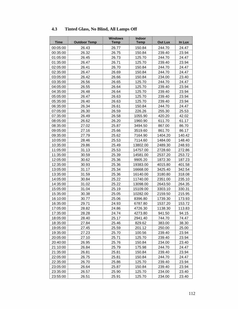
112

4.3 Tinted Glass, No Blind, All Lamps Off

Time Outdoor Temp Windows


00:05:00 26.43 26.77 150.84 244.70 24.47 00:35:00 26.32 26.75 150.84 239.40 23.94 01:05:00 26.45 26.73 125.70 244.70 24.47 01:35:00 26.47 26.71 125.70 239.40 23.94 02:05:00 26.41 26.70 150.84 244.70 24.47 02:35:00 26.47 26.69 150.84 244.70 24.47 03:05:00 26.42 26.66 150.84 234.00 23.40 03:35:00 26.56 26.65 125.70 244.70 24.47 04:05:00 26.55 26.64 125.70 239.40 23.94 04:35:00 26.48 26.64 125.70 239.40 23.94 05:05:00 26.47 26.63 125.70 239.40 23.94 05:35:00 26.40 26.63 125.70 239.40 23.94 06:35:00 26.34 26.61 150.84 244.70 24.47 07:05:00 26.30 26.59 226.26 255.30 25.53 07:35:00 26.49 26.58 1055.90 420.20 42.02 08:05:00 26.62 26.20 1960.90 611.70 61.17 08:35:00 27.02 25.87 3494.50 867.00 86.70 09:05:00 27.16 25.66 3519.60 861.70 86.17 09:35:00 27.79 25.62 7164.90 1404.20 140.42 10:05:00 28.46 25.53 7114.60 1484.00 148.40 10:35:00 29.86 25.49 13802.00 2489.30 248.93 11:05:00 31.13 25.53 14757.00 2728.60 272.86 11:35:00 30.59 25.39 14581.00 2537.20 253.72 12:05:00 30.62 25.36 9905.20 1872.30 187.23 12:35:00 30.93 25.36 19383.00 4015.80 401.58 13:05:00 31.17 25.34 16668.00 3425.40 342.54 13:35:00 31.59 25.36 16140.00 3180.80 318.08 14:05:00 30.84 25.22 11740.00 2351.00 235.10 14:35:00 31.02 25.22 13098.00 2643.50 264.35 15:05:00 31.04 25.19 15109.00 3303.10 330.31 15:35:00 30.38 25.05 10282.00 2159.50 215.95 16:10:00 30.77 25.06 8396.80 1739.30 173.93 16:35:00 29.71 24.93 6787.80 1537.20 153.72 17:05:00 28.82 24.86 4726.30 1138.30 113.83 17:35:00 28.28 24.74 4273.80 941.50 94.15 18:05:00 28.40 25.17 2941.40 744.70 74.47 18:35:00 27.84 25.46 829.62 383.00 38.30 19:05:00 27.45 25.59 201.12 250.00 25.00 19:35:00 27.23 25.70 100.56 239.40 23.94 20:05:00 27.10 25.71 125.70 239.40 23.94 20:40:00 26.95 25.76 150.84 234.00 23.40 21:10:00 26.84 25.79 175.98 244.70 24.47 21:35:00 26.81 25.81 150.84 239.40 23.94 22:05:00 26.75 25.81 150.84 244.70 24.47 22:35:00 26.70 25.86 125.70 239.40 23.94 23:05:00 26.64 25.87 150.84 239.40 23.94 23:35:00 26.57 25.90 125.70 234.00 23.40 23:55:00 26.51 25.91 125.70 234.00 23.40

113

0

5

10

15

20

25

30

35

00:00:00 04:48:00 09:36:00 14:24:00 19:12:00 00:00:00 04:48:00

Outdoor TempWindows Temp


on the window and the lamps is off

0

500

1000

1500

2000

2500

3000

3500

4000

4500

00:00:00 04:48:00 09:36:00 14:24:00 19:12:00 00:00:00 04:48:00

Out LuxIn Lux

Graphic. 4. Outdoor lux and indoor lux when there is no blind in on the

window and the lamps is off

114

4.4 Tinted Glass, With Blind, All Lamps On



00:05:00 24.42 25.37 25.77 125.70 273.93 00:35:00 24.05 25.48 25.77 125.70 275.52 01:05:00 25.05 25.42 25.78 100.56 277.12 01:35:00 23.56 25.52 25.78 125.70 276.06 02:05:00 23.55 25.56 25.79 150.84 277.12 02:35:00 24.20 25.54 25.76 125.70 278.18 03:05:00 24.50 25.50 25.80 150.84 276.06 03:35:00 25.17 25.57 25.79 125.70 275.52 04:05:00 25.24 25.56 25.80 125.70 276.06 04:35:00 24.77 25.49 25.80 125.70 276.06 05:05:00 23.95 25.32 25.82 125.70 276.59 05:35:00 24.81 25.39 25.85 175.98 276.06 06:05:00 24.62 25.40 25.85 125.70 278.18 06:35:00 24.53 25.39 25.86 125.70 278.18 07:05:00 24.64 25.41 25.86 251.40 277.65 07:35:00 25.18 25.56 25.89 653.64 282.97 08:05:00 25.24 25.85 25.90 1508.40 287.23 08:35:00 25.77 26.24 25.92 2086.60 292.01 09:05:00 25.94 26.59 25.94 3318.50 303.18 09:35:00 28.33 28.84 26.01 12319.00 373.39 10:05:00 28.13 31.54 26.18 12143.00 365.95 10:35:00 26.74 30.76 26.26 11187.00 361.69 11:05:00 26.90 29.72 26.18 8623.00 342.54 11:35:00 28.44 29.90 26.04 9100.70 348.39 12:05:00 29.60 29.80 26.08 8069.90 341.48 12:35:00 29.65 29.83 26.07 8924.70 346.80 13:05:00 30.91 30.36 26.04 10584.00 357.44 13:35:00 30.71 31.00 26.17 11564.00 366.48 14:05:00 31.67 31.29 26.12 11011.00 363.29 14:35:00 31.26 31.02 26.19 9352.10 352.12 15:05:00 29.66 30.46 26.21 8698.40 347.33 15:35:00 29.34 30.16 26.18 7692.80 330.31 16:05:00 30.54 29.95 26.28 7039.20 326.05 16:35:00 30.41 30.25 26.22 7089.50 329.25 17:05:00 30.77 30.55 26.30 6963.80 329.78 17:35:00 30.57 29.68 26.29 3796.10 302.12 18:05:00 29.80 28.81 26.39 1759.80 288.82 18:35:00 29.12 28.19 26.50 729.06 274.46 19:05:00 28.53 27.72 26.54 125.70 272.86 19:35:00 27.63 27.53 26.61 125.70 271.80 20:05:00 28.05 27.45 26.65 125.70 272.86 20:35:01 27.95 27.36 26.70 125.70 271.27 21:05:00 27.79 27.28 26.74 125.70 271.27 21:35:00 27.60 27.21 26.77 125.70 270.21 22:05:00 27.66 27.20 26.80 125.70 272.33 22:35:00 27.50 27.26 26.84 125.70 269.14 23:05:00 27.19 27.19 26.83 125.70 270.74 23:35:00 27.30 27.11 26.83 125.70 272.86 23:55:00 27.47 27.11 26.83 150.84 272.86

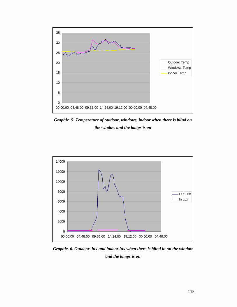
115

0

5

10

15

20

25

30

35

00:00:00 04:48:00 09:36:00 14:24:00 19:12:00 00:00:00 04:48:00


Graphic. 5. Temperature of outdoor, windows, indoor when there is blind on

the window and the lamps is on

0

2000

4000

6000

8000

10000

12000

14000

00:00:00 04:48:00 09:36:00 14:24:00 19:12:00 00:00:00 04:48:00

Out LuxIn Lux

Graphic. 6. Outdoor lux and indoor lux when there is blind in on the window

and the lamps is on

116

4.5 Tinted Glass, With Blind, All Lamps Off



00:00:00 27.39 27.69 27.82 175.98 255.30 01:05:00 27.46 27.60 27.82 201.12 250.00 01:35:00 27.30 27.56 27.81 201.12 250.00 02:05:00 26.90 27.45 27.80 175.98 250.00 02:35:00 26.98 27.43 27.79 175.98 250.00 03:05:00 26.74 27.35 27.78 175.98 255.30 03:35:00 26.43 27.23 27.76 175.98 250.00 04:05:00 26.58 27.19 27.75 175.98 260.60 04:35:00 26.37 27.12 27.74 150.84 250.00 05:05:00 26.17 27.05 27.73 175.98 255.30 05:35:00 26.22 27.04 27.71 175.98 255.30 06:05:00 26.26 27.00 27.69 150.84 250.00 06:35:00 26.23 26.94 27.68 175.98 250.00 07:05:00 26.22 26.96 27.66 553.08 287.20 07:35:00 26.62 27.37 27.66 1860.40 383.00 08:35:00 32.63 31.94 27.14 33637.00 1718.00 09:05:00 34.84 36.02 27.05 11715.00 1579.70 09:35:00 33.36 33.01 26.92 8170.50 776.60 10:05:00 33.52 32.69 26.69 8623.00 898.90 10:35:00 33.59 32.36 26.65 11313.00 1106.40 11:05:00 34.13 32.64 26.59 13827.00 1372.30 11:35:00 33.27 32.40 26.52 16190.00 1563.80 12:05:00 31.76 31.97 26.52 11992.00 1228.70 12:35:00 34.30 33.68 26.66 16014.00 1553.10 13:05:00 32.10 32.39 26.58 12947.00 1276.60 13:35:00 31.99 32.07 26.54 11363.00 1164.90 14:05:00 32.16 31.65 26.45 8447.00 936.10 14:35:00 31.35 30.98 26.37 7039.20 824.40 15:05:00 32.55 31.04 26.31 7164.90 835.10 15:35:00 31.43 30.39 26.24 6838.10 792.50 16:05:00 30.86 31.06 26.25 7919.10 867.00 16:35:01 31.84 30.49 26.20 5656.50 707.40 17:05:00 30.75 29.84 26.12 4650.90 606.40 17:35:00 30.55 29.39 26.06 3771.00 547.90 18:05:00 31.07 29.80 26.54 3544.70 547.90 18:35:00 29.89 28.99 26.77 854.76 324.50 19:05:00 29.80 28.46 26.82 276.54 255.30 19:35:00 29.34 28.10 26.84 201.12 244.70 20:05:00 28.77 27.87 26.86 201.12 260.60 20:35:00 28.53 27.73 26.90 201.12 250.00 21:05:00 28.21 27.61 26.93 201.12 255.30 21:35:00 27.96 27.51 26.95 201.12 244.70 22:05:00 27.55 27.41 26.97 175.98 250.00 22:35:00 27.60 27.34 26.95 175.98 250.00 23:05:00 27.32 27.29 26.96 175.98 255.30 23:35:00 27.30 27.21 26.97 175.98 255.30 23:55:00 27.27 27.18 26.96 175.98 255.30

117

0.00

5.00

10.00

15.00

20.00

25.00

30.00

35.00

40.00

0 10 20 30 40 50 60


Graphic. 7. Temperature of outdoor, windows, indoor when there is blind on

the window and the lamps is off

0.00

5000.00

10000.00

15000.00

20000.00

25000.00

30000.00

35000.00

40000.00

0 10 20 30 40 50 60

Out LuxIn Lux

Graphic. 8. Outdoor lux and indoor lux when there is blind on the window and

the lamps is off

118

4.6 Tinted glass, No blind, All Lamps On, AC On

Time Outdoor

Temp Windows

Temp Indoor Temp Out Lux In Lux 00:00:00 26.57 26.45 25.27 281.91 125.70 00:35:00 26.31 25.38 25.29 283.50 100.56 01:05:00 26.45 26.40 25.30 281.91 125.70 01:35:00 26.31 26.35 25.31 282.44 125.70 02:05:00 26.26 26.37 25.33 283.50 100.56 02:35:01 25.83 26.25 25.34 280.84 125.70 03:05:00 26.11 26.34 25.35 281.38 150.84 03:35:00 26.06 26.31 25.36 281.91 150.84 04:05:00 25.99 26.34 25.37 280.31 150.84 04:35:00 26.07 26.31 25.38 281.38 150.84 05:05:00 25.98 26.29 25.38 281.38 125.70 05:35:00 25.78 26.16 25.38 285.10 125.70 06:05:00 25.62 26.15 25.39 283.50 125.70 06:35:00 25.71 26.14 25.38 280.84 125.70 07:35:00 26.34 26.53 25.36 298.40 1759.80 08:05:00 27.10 26.80 25.00 317.01 2690.00 08:35:00 34.22 29.46 24.89 443.07 39470.00 09:05:00 31.34 31.33 24.86 395.73 6134.20 09:35:00 32.20 29.81 24.71 403.71 7642.60 10:05:00 32.48 30.11 24.73 404.78 7944.20 10:35:00 32.27 30.22 24.62 469.14 11388.00 11:05:00 31.34 29.50 24.63 478.71 11539.00 11:35:00 31.96 29.54 24.53 502.11 12872.00 12:05:00 33.52 30.72 24.63 464.35 11439.00 12:35:00 33.90 31.19 24.60 534.03 13676.00 13:05:00 32.69 30.71 24.56 547.86 14833.00 13:35:01 32.77 31.28 24.62 447.86 10207.00 14:05:00 32.87 30.96 24.53 392.01 7315.70 14:10:00 32.58 30.62 24.51 381.90 6662.10 14:15:00 32.60 30.33 24.52 379.78 6435.80 14:25:00 32.88 29.99 24.53 384.56 7014.10 14:30:00 32.54 29.89 24.53 379.24 6435.80 14:35:00 32.52 29.79 24.51 370.20 5656.50 15:05:00 33.11 29.75 24.43 484.03 11238.00 16:05:00 32.19 30.31 24.53 322.33 2287.70 16:35:00 28.01 27.39 25.40 291.48 603.36 17:05:00 27.66 26.71 25.27 288.29 326.82 17:35:00 27.59 26.57 25.25 287.23 527.94 18:05:00 27.83 26.65 25.46 289.35 402.24 18:35:00 27.87 26.71 25.66 285.63 251.40 19:05:00 27.42 26.71 25.78 284.57 150.84 19:35:00 27.39 26.71 25.88 281.38 100.56 20:35:00 27.38 26.71 25.98 283.50 125.70 21:05:00 27.26 26.78 26.03 280.84 150.84 21:35:00 27.35 26.69 26.07 280.31 150.84 22:05:00 27.12 26.61 26.09 282.97 125.70 22:35:00 26.96 26.58 26.12 284.03 100.56 23:05:00 26.82 26.51 26.15 282.97 125.70 23:55:00 26.63 26.47 26.20 284.57 125.70

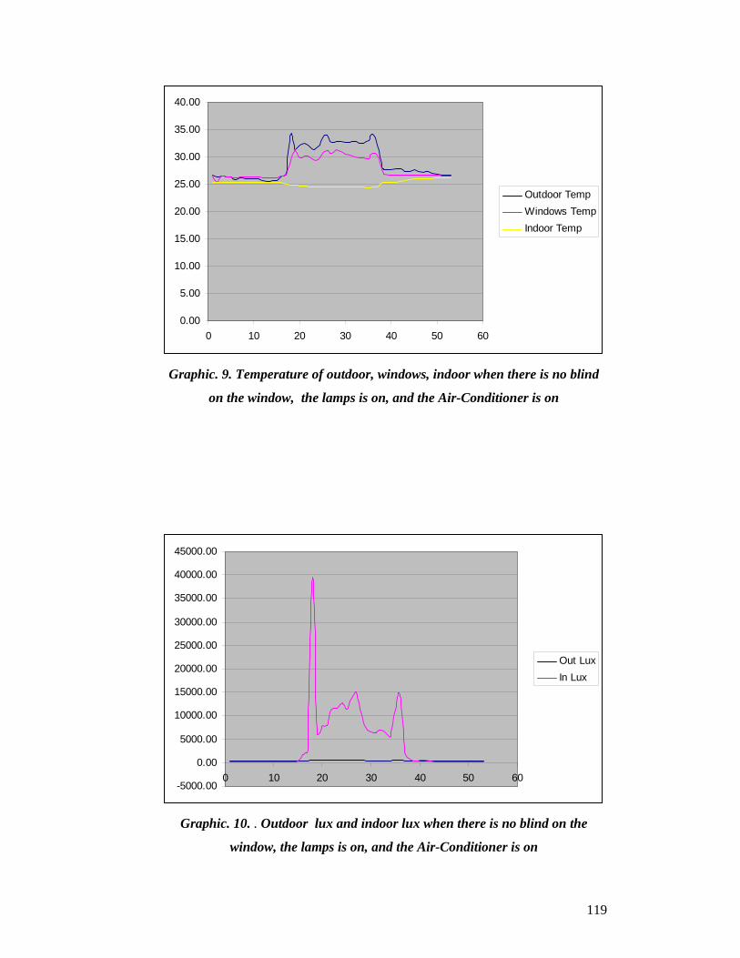
119

0.00

5.00

10.00

15.00

20.00

25.00

30.00

35.00

40.00

0 10 20 30 40 50 60



on the window, the lamps is on, and the Air-Conditioner is on

-5000.00

0.00

5000.00

10000.00

15000.00

20000.00

25000.00

30000.00

35000.00

40000.00

45000.00

0 10 20 30 40 50 60

Out LuxIn Lux

Graphic. 10. . Outdoor lux and indoor lux when there is no blind on the

window, the lamps is on, and the Air-Conditioner is on

120

CHAPTER V

CONCLUSION AND RECOMMENDATION

5.1. Conclusion

Generally, project’s objective to design a control circuit that controls the

operation of an air conditioner automatically and manually has been achieved. In this

project, the control circuit is called ‘Programmable Thermostat’. Even though there are

already programmable thermostats created in market, but this one is different. It only

consists of a circuit which acts more like a switch in order to on and off the compressor.

Method of control depends on the user to choose whether the compressor functions

automatically or manually.

Through systematic usage of the compressor, the cooling load can be reduced

and thus, energy can be conserved. Air conditioner will operate economically by using a

proper control system. Instead of just air conditioner, this control circuit can also be

used in controlling other electrical appliances such as television, lighting and others.

By combining automatic window blind controller with lighting controller, the

performance of the energy saving is increased. Automatic window blind controller is

used to control the sunlight infiltration while the lighting controller is operated when the

intensity of the room is not adequate to the standard lux of the room. By combining this

system, the optimum energy saving is achieved.

121

5.2. Recommendation

Implementing fuzzy logic controller into this project would make it more

efficient and easier. Fuzzy logic is one of the Artificial Intelligence Control Design

Techniques and it is widely used as controller throughout the world. Many industrial

and consumer products using fuzzy logic technology have been built, especially in

Japan. There are different incentives to use fuzzy logic. Among them are:

a) Industrial AC systems use fuzzy logic to minimize energy consumption. The

implementation of complex control strategies optimizes that the set values for

the heater, cooler, and humidifier shall be set in a certain load state

b) Car AC systems use fuzzy logic to estimate the temperatures at the head of the

driver from multiple indirect sensors.

c) Home AC systems are much simpler. They do not contain a humidifier and can

only either cool or heat at one time. They use fuzzy logic for robust temperature

control.

If using fuzzy logic, inputs and output are needed. In this case, fuzzy logic

system uses four input variables which are:

a) Difference between set and room temperature (Temp_Error).

When the difference between set temperature and room temperature is very

large, the fuzzy logic system increases the signal so the desired temperature is

reached faster

b) Time differentiated set temperature (dTemp_by_dt)

The set temperature signal is differentiated with a time constant of 30 minutes.

The fuzzy logic system uses this signal to understand when the user wants the

AC to cool down a room quick

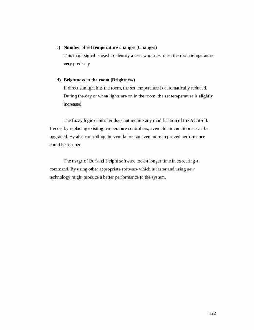
122

c) Number of set temperature changes (Changes)

This input signal is used to identify a user who tries to set the room temperature

very precisely

d) Brightness in the room (Brightness)

If direct sunlight hits the room, the set temperature is automatically reduced.

During the day or when lights are on in the room, the set temperature is slightly

increased.

The fuzzy logic controller does not require any modification of the AC itself.

Hence, by replacing existing temperature controllers, even old air conditioner can be

upgraded. By also controlling the ventilation, an even more improved performance

could be reached.

The usage of Borland Delphi software took a longer time in executing a

command. By using other appropriate software which is faster and using new

technology might produce a better performance to the system.

Reference

1. E.S. Lee, D.L. DiBartolomeo, S.E. Selkowitz, “Thermal and Daylighting

Performance of An Automated Venetian Blind and Lighting System in A Full-

Scale Private Office”, Energy and Buildings 29 (1998) 47-63, Elsevier

Science, 1998.

2. H. B. Kuntze and Th. Bernard, “A New Fuzzy-based Supervisory Control

Concept for the Demand-responsive Optimization of HVAC Control

Systems”, Proceeding of the 37th IEEE Conference on Decision & Control,

FM16 12:10, Tampa Florida, USA, 1998.

3. Jabatan Kerja Raya (JKR) Malaysia, “Illumination Standard”.

4. Maher Hamdi, Gérard Lachiver, “A Fuzzy Control System Based on The

Human Sensation of Thermal Comfort”, IEEE Transaction, 0-7803-4863-

X/98, 1998.

5. M. M. Eftekhari, L. D. Marjanovic, “ Application of Fuzzy Control in

Naturally Ventilated Buildings for Summer Conditions”, Energy and

Buildings 35(2003) 645-655, Elsevier Science, 2002.

6. Robert N. Lea, Edgar Dohmann, Wayne Prebilsky, Yashvant Jani, “An HVAC

Fuzzy Logic Zone Control System and Performance Results”, IEEE

Transaction 0-7803-3645-3/96, 1996.

7. Saiful Jamaan, Md Shah Majid, Mohd Wazir Mustafa, Hasimah Abd Rahman,

“A PC based Fuzzy Logic Power System Stabilizer”, Seminar on Artificial

Intelligence Applications in Industry, AIAI 2003, A Collaborative Effort

between Malaysia and Japan, Kuala Lumpur 24-25 June 2003.

8. Thomas E. Kissel, “Electricity, Electronics, And Control Systems for HVAC,

Prentice Hall, ISBN: 0-13-011988-1, 2000.

9. Mohd. Aizly Bin Mohammad Noh, “Programmable Thermostat”, Dissertation

for Bachelor of Electrical Engineering, Universiti Teknologi Malaysia,

Skudai, May 2006.

10. Paul Paran Puloh, “Sistem Tingkap Automatik”, Dissertation for Bachelor of

Electrical Engineering, Universiti Teknologi Malaysia, Skudai, May 2006.

VOT 74120 DEVELOPMENT OF AN ON-LINE AND … · sektor komersil telah menggunakan 19 peratus...

Documents

Transcript of VOT 74120 DEVELOPMENT OF AN ON-LINE AND … · sektor komersil telah menggunakan 19 peratus...