Sains Malaysiana 45(11)(2016): 1625–1633

Evaluation Performance of Time Series Approach for Forecasting Air Pollution Index in Johor, Malaysia

(Penilaian Prestasi Pendekatan Siri Masa untuk Peramalan Indeks Pencemaran Udara di Johor, Malaysia)

NUR HAIZUM ABD RAHMAN, MUHAMMAD HISYAM LEE*, SUHARTONO & MOHD TALIB LATIF

ABSTRACT

The air pollution index (API) has been recognized as one of the important air quality indicators used to record the correlation between air pollution and human health. The API information can help government agencies, policy makers and individuals to prepare precautionary measures in order to eliminate the impact of air pollution episodes. This study aimed to verify the monthly API trends at three different stations in Malaysia; industrial, residential and sub-urban areas. The data collected between the year 2000 and 2009 was analyzed based on time series forecasting. Both classical and modern methods namely seasonal autoregressive integrated moving average (SARIMA) and fuzzy time series (FTS) were employed. The model developed was scrutinized by means of statistical performance of root mean square error (RMSE). The results showed a good performance of SARIMA in two urban stations with 16% and 19.6% which was more satisfactory compared to FTS; however, FTS performed better in suburban station with 25.9% which was more pleasing compared to SARIMA methods. This result proved that classical method is compatible with the advanced forecasting techniques in providing better forecasting accuracy. Both classical and modern methods have the ability to investigate and forecast the API trends in which can be considered as an effective decision-making process in air quality policy.

Keywords: Air pollution index; ARIMA; forecasting; fuzzy time series; time series

ABSTRAK

Indeks pencemaran udara (IPU) penting sebagai petunjuk asas kualiti udara yang berkait rapat antara pencemaran udara dan kesihatan manusia. Maklumat IPU boleh membantu agensi kerajaan, penggubal dasar serta orang perseorangan untuk menyediakan langkah berjaga-jaga untuk mengatasi pencemaran udara. Kajian ini bertujuan untuk menganalisis trend IPU bulanan di tiga buah stesen yang berbeza di Malaysia; industri, perumahan dan pinggir bandar. Data antara tahun 2000 dan 2009 telah dianalisis berdasarkan siri ramalan masa. Kedua-dua kaedah klasik dan moden iaitu autoregresif bermusim bersepadu purata (SARIMA) dan siri masa kabur (FTS) telah diaplikasikan. Model ramalan dibandingkan melalui prestasi statistik punca min ralat kuasa dua (RMSE). Hasil kajian menunjukkan SARIMA meramal dengan baik di dua stesen bandar dengan 16% dan 19.6% yang lebih memuaskan berbanding FTS; Walau bagaimanapun, ramalan FTS lebih baik di stesen pinggir bandar dengan 25.9% lebih tepat berbanding dengan kaedah SARIMA. Keputusan ini membuktikan bahawa kaedah klasik mampu meramal dengan baik standing dengan teknik ramalan yang moden. Kedua-dua kaedah klasik dan moden mempunyai keupayaan untuk mengkaji dan meramal trend IPU dan boleh membantu dalam proses membuat keputusan yang berkesan dalam membentuk dasar kualiti udara.

Kata kunci: ARIMA; indeks pencemaran udara; ramalan; siri masa; siri masa kabur

INTRODUCTION

The presence of globalized development for both developed and developing countries has contributed to the increase of pollution problems (Hassanzadeh et al. 2009). Air pollution is the most prevalent type of pollution in the world and is predominantly caused by natural activities such as volcano eruptions and human-based factors, for example, open burning and industrial processes (Afroz et al. 2003; Kurt & Oktay 2010; Wang & Lu 2006). However, fuel burning vehicles are the main reason for air pollution to increase and this is particularly true in urban areas (Afroz et al. 2003; Wang & Lu 2006).

Air pollution has been affecting human health and the environment; and in the long-term it tends to exacerbate the risks to earth, by increasing global warming due to the greenhouse effect (Heo & Kim 2004; Kumar & Jain 2010; Kurt & Oktay 2010). In order to assess the impact of air quality status on human health, a simple generalized method which combines the API, scale and terms has been used for several years (Kumar & Goyal 2011). The API in Malaysia was developed based on the API introduced by the United State Environmental Protection Agency (USEPA) and is determined by calculating the sub-indexes of the five main pollutants, namely particulate matter

1626

(PM10), ozone (O3), carbon monoxide (CO2), sulphur dioxide (SO2) and nitrogen dioxide (NO2). The highest value among these sub-indexes is then chosen as the API for the time of interest. According to the Department of Environment (DoE) (2005), in Malaysia, different categories of sub-indexes represent different effects on human health. Air quality forecasting is reliable and effective in controlling the measures and can be suggested as a preventive and evasive action for regulations that are to be enforced (Kumar & Goyal 2011; Nurulilyana et al. 2011). In the time series, historical observations are analyzed to develop a model that describes the relationship between time and variables and this will be used to extrapolate the time series in the future (Cryer 1986). This approach has been adopted for air quality management to help future planning and to seek ways to improve air quality. With regards to air quality, lots of research has been conducted, predominantly focusing on monitoring the main pollutants: PM10, O3, CO2, SO2, and NO2 (Brunelli et al. 2007; Chaloulakou et al. 2003; Kumar & Jain 2010; Nurul Adyani et al. 2010; Vlachogianni et al. 2011). Realizing the importance of API and air quality forecasting, this study aimed to focus on the prediction of monthly mean API using the time series model. Whilst the Box-Jenkins has been commonly used for years to predict pollutants and API data sets (Hassanzadeh et al. 2009; Kumar & Jain 2010; Nurulilyana et al. 2011; Nurul Adyani et al. 2010; Wang & Lu 2006), these conventional methods have some limitations regarding the linearity and stationary assumptions are needed. Recently, new forecasting techniques have led to the improvement of forecasting accuracy (Khashei & Bijari 2010). Thus, FTS will be introduced to model and forecast the API data.

METHODS

DESCRIPTION OF THE SAMPLING SITE

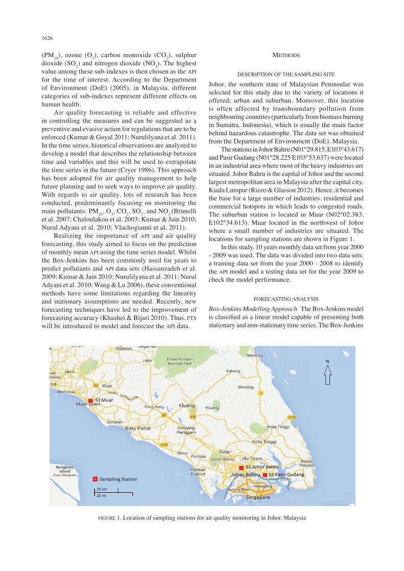
Johor, the southern state of Malaysian Peninsular was selected for this study due to the variety of locations it offered; urban and suburban. Moreover, this location is often affected by transboundary pollution from neighbouring countries (particularly from biomass burning in Sumatra, Indonesia), which is usually the main factor behind hazardous catastrophe. The data set was obtained from the Department of Environment (DoE), Malaysia. The stations in Johor Bahru (N01°29.815, E103°43.617) and Pasir Gudang (N01°28.225 E103°53.637) were located in an industrial area where most of the heavy industries are situated. Johor Bahru is the capital of Johor and the second largest metropolitan area in Malaysia after the capital city, Kuala Lumpur (Rizzo & Glasson 2012). Hence, it becomes the base for a large number of industries, residential and commercial hotspots in which leads to congested roads. The suburban station is located in Muar (N02°02.383, E102°34.613). Muar located in the northwest of Johor where a small number of industries are situated. The locations for sampling stations are shown in Figure 1. In this study, 10 years monthly data set from year 2000 - 2009 was used. The data was divided into two data sets; a training data set from the year 2000 - 2008 to identify the API model and a testing data set for the year 2009 to check the model performance.

FORECASTING ANALYSIS

Box-Jenkins Modelling Approach The Box-Jenkins model is classified as a linear model capable of presenting both stationary and non-stationary time series. The Box-Jenkins

FIGURE 1. Location of sampling stations for air quality monitoring in Johor, Malaysia

1627

method is inclusive of three main models; autoregressive (AR), integrated (I) models and moving average (MA). The AR and MA models are suitable for stationary time series pattern and the mixture of AR and MA could obtain the ARMA models whilst for non-stationary data set, I models could make the data set stationary to obtain ARIMA models (Cryer 1986). Tentative identification, parameter estimation and diagnostic checking are the important procedures in determining the best model for time series data (Hanke & Wichern 2005). Since the API data that we used was measured at regular calendar intervals in a year, it may exhibit periodic behaviour. In this case, where the seasonal components are included, the model is referred to as a seasonal ARIMA model or SARIMA model. The model can be abbreviated to SARIMA (p, d, q)(P, D, Q)S where the lowercase letters represent the non-seasonal part whilst the uppercase letters show the seasonal part (Muhammad Hisyam et al. 2012). The generalized form of SARIMA model can be written as:

ϕp(B)Фp(BS)(1 – B)d(1–BS)DYt = θq(B)ΘQ(BS)εt (1)

where,

ϕp(B) = 1 – ϕ1B – ϕ2B2 – … – ϕpB

p; Фp(B)

= 1 – Ф1BS – Ф2B

2S – … – ФpBPS;

θq(B) = 1 – θ1B – θ2B2 – … – θpB

p; ФQ(B)

= 1 – Ф1BS – Ф2B

2S – … – ФQBQS;

Fuzzy Time Series Analysis The FTS series have been used in the field of air pollution by several authors (Heo & Kim 2004). According to Song and Chissom (1993a, 1993b), generally, the concepts of FTS can be defined as: let U be the universe of discourse, where U = {u1, u2, …, ub} and U = [Dmin – D1, Dmax +D2] = [begin, end]. A fuzzy set (Ai) of U is defined as Ai = fA1(u1)/u1 + fA1(u2) + … + fAi(ub)/ub, where fAi is the membership function of the fuzzy set A, fA: U →[0,1]. ua is a generic element of fuzzy set A1, and fAi(ua) is the grade of membership of ua in Ai, where fAi(ua) ∈[0,1] and 1 ≤ a ≤ b. Based on Song and Chissom’s (1993a, 1993b,) work, Chen (1996) improved the establishment step of fuzzy relationships with a simple operation instead of complex matrix operations. In Chen (1996), the repeated or the recent identical fuzzy logical relationships (FLRs) were simply ignored since the same FLR may not reflect the real world situation. For example,

(t = 1) A1→ A1, (t = 2) A1 → A2, (t = 3) A1 → A1,

(t = 4) A1 → A1.

As shown in the above FLR, Chen method ignores the relationship between (t = 3) and (t = 4). Therefore, the fuzzy logical relationship group (FLRG) is left as A1 → A1, A2.

In contrast, Yu (2005) proposed that the same FLR must be considered in forecasting since the recent FLR has greater weight. Therefore, the probability of its appearance in the future is higher. To illustrate, the Yu FTS can be shown as:

(t = 1) A1 → A1 with weight 1, (t = 2) A1 → A2 with weight 2, (t = 3) A1 → A1 with weight 3, (t = 4) A1 → A1 with weight 4.

As shown before, the most recent FLR (t = 4) is assigned with the highest weight of 4 indicating high probability of its occurrence in the future. Conversely, the initial FLR (t = 1) is assigned with the lowest weight of 1, thus indicates the lowest probability compared to other FLRs. Instead, Cheng et al. (2008) proposed the probability of weight appearance and the importance of chronological FLR for the same recent identical FLRS. The weights can be illustrated as follows:

(t = 1) A1 → A1 with weight 1, (t = 2) A1 → A2 with weight 1, (t = 3) A1 → A1 with weight 2, (t = 4) A1 → A1 with weight 3.

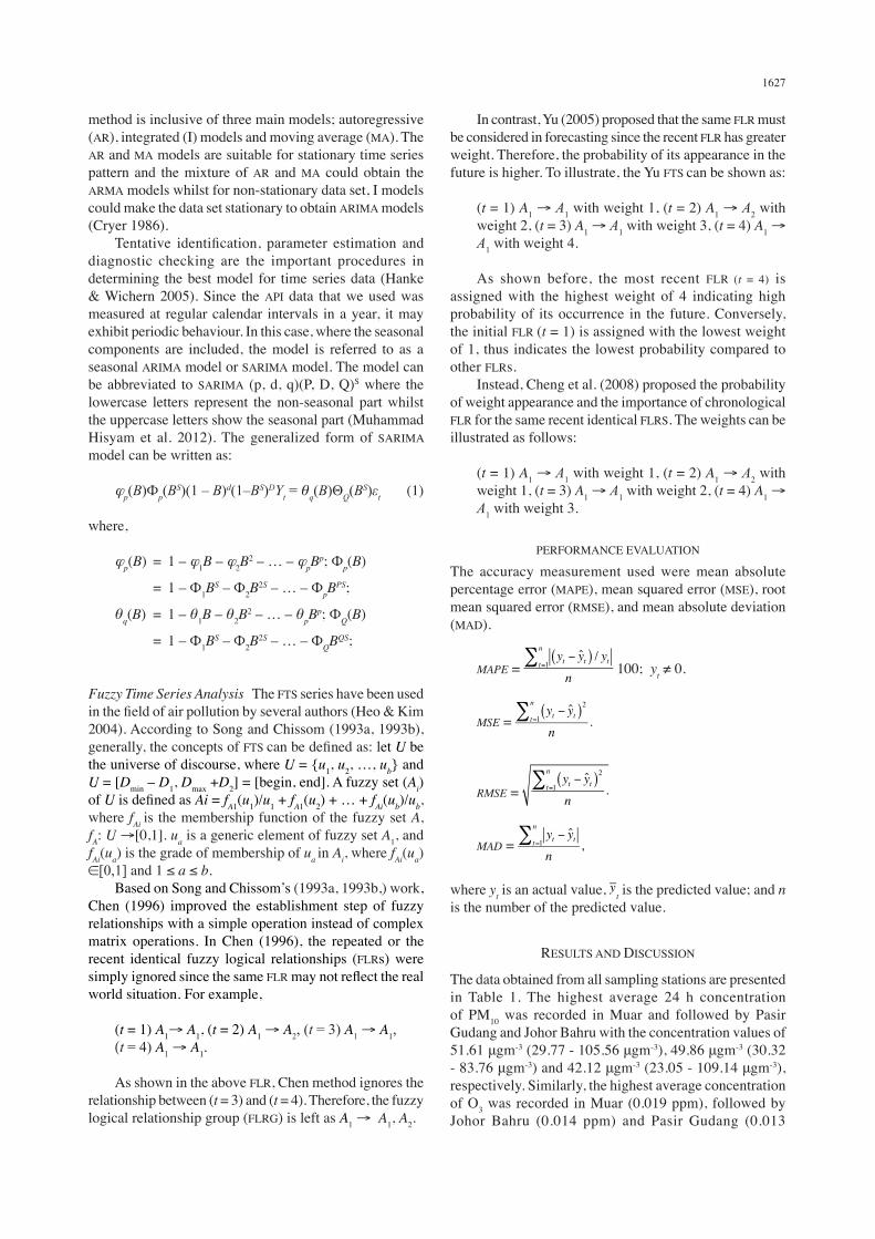
PERFORMANCE EVALUATION

The accuracy measurement used were mean absolute percentage error (MAPE), mean squared error (MSE), root mean squared error (RMSE), and mean absolute deviation (MAD).

MAPE = 100; yt ≠ 0.

MSE =

RMSE =

MAD =

where yt is an actual value, t is the predicted value; and n is the number of the predicted value.

RESULTS AND DISCUSSION

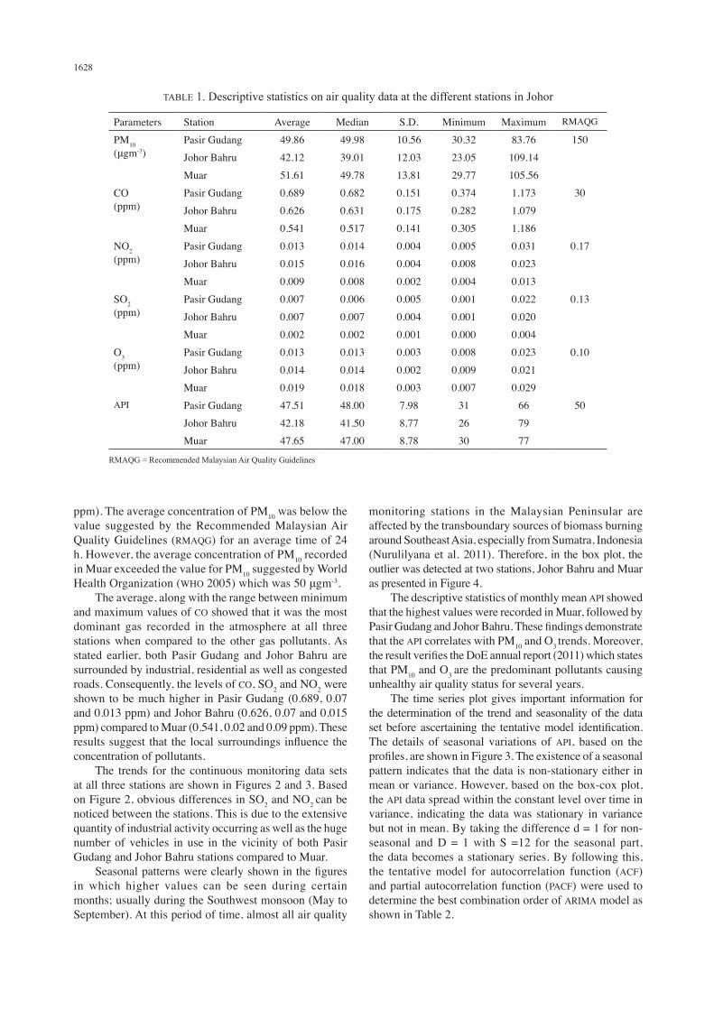
The data obtained from all sampling stations are presented in Table 1. The highest average 24 h concentration of PM10 was recorded in Muar and followed by Pasir Gudang and Johor Bahru with the concentration values of 51.61 μgm-3 (29.77 - 105.56 μgm-3), 49.86 μgm-3 (30.32 - 83.76 μgm-3) and 42.12 μgm-3 (23.05 - 109.14 μgm-3), respectively. Similarly, the highest average concentration of O3 was recorded in Muar (0.019 ppm), followed by Johor Bahru (0.014 ppm) and Pasir Gudang (0.013

1628

ppm). The average concentration of PM10 was below the value suggested by the Recommended Malaysian Air Quality Guidelines (RMAQG) for an average time of 24 h. However, the average concentration of PM10 recorded in Muar exceeded the value for PM10 suggested by World Health Organization (WHO 2005) which was 50 μgm-3. The average, along with the range between minimum and maximum values of CO showed that it was the most dominant gas recorded in the atmosphere at all three stations when compared to the other gas pollutants. As stated earlier, both Pasir Gudang and Johor Bahru are surrounded by industrial, residential as well as congested roads. Consequently, the levels of CO, SO2 and NO2 were shown to be much higher in Pasir Gudang (0.689, 0.07 and 0.013 ppm) and Johor Bahru (0.626, 0.07 and 0.015 ppm) compared to Muar (0.541, 0.02 and 0.09 ppm). These results suggest that the local surroundings influence the concentration of pollutants. The trends for the continuous monitoring data sets at all three stations are shown in Figures 2 and 3. Based on Figure 2, obvious differences in SO2 and NO2 can be noticed between the stations. This is due to the extensive quantity of industrial activity occurring as well as the huge number of vehicles in use in the vicinity of both Pasir Gudang and Johor Bahru stations compared to Muar. Seasonal patterns were clearly shown in the figures in which higher values can be seen during certain months; usually during the Southwest monsoon (May to September). At this period of time, almost all air quality

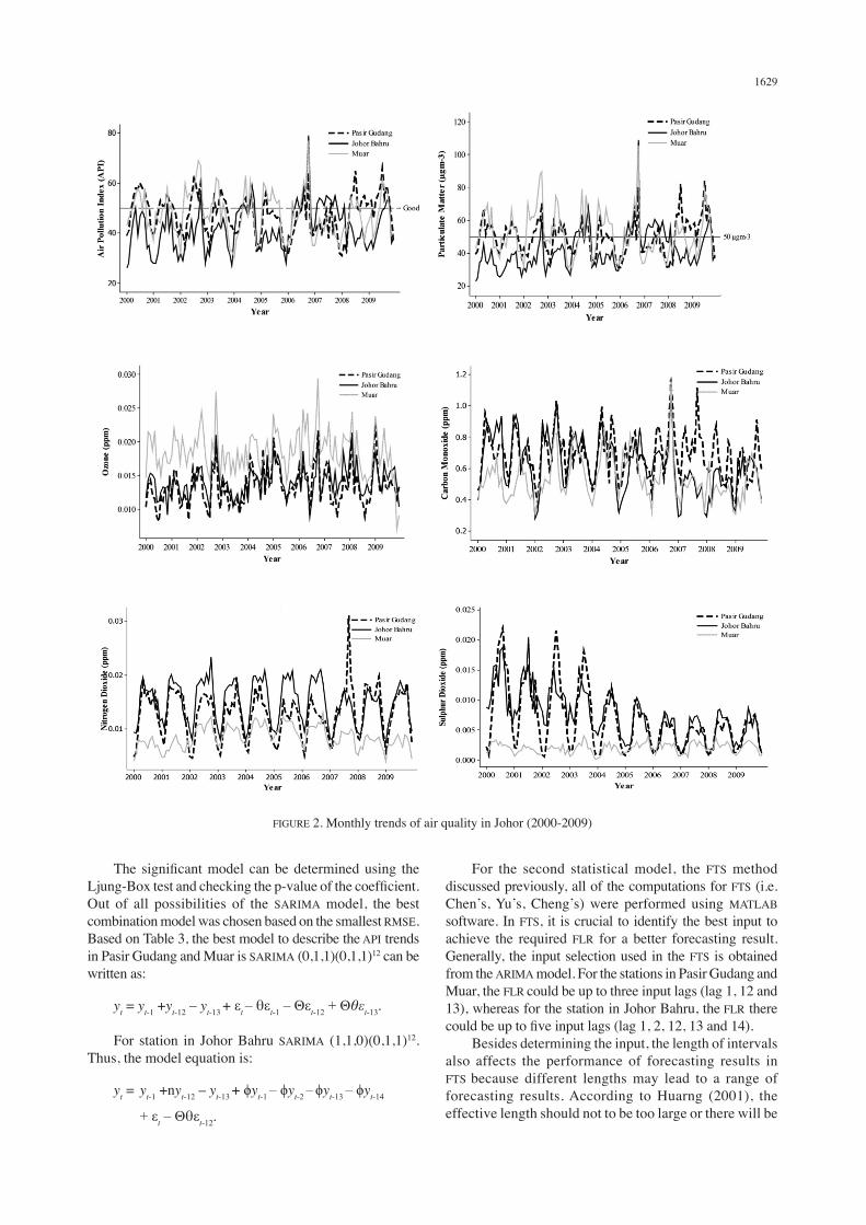
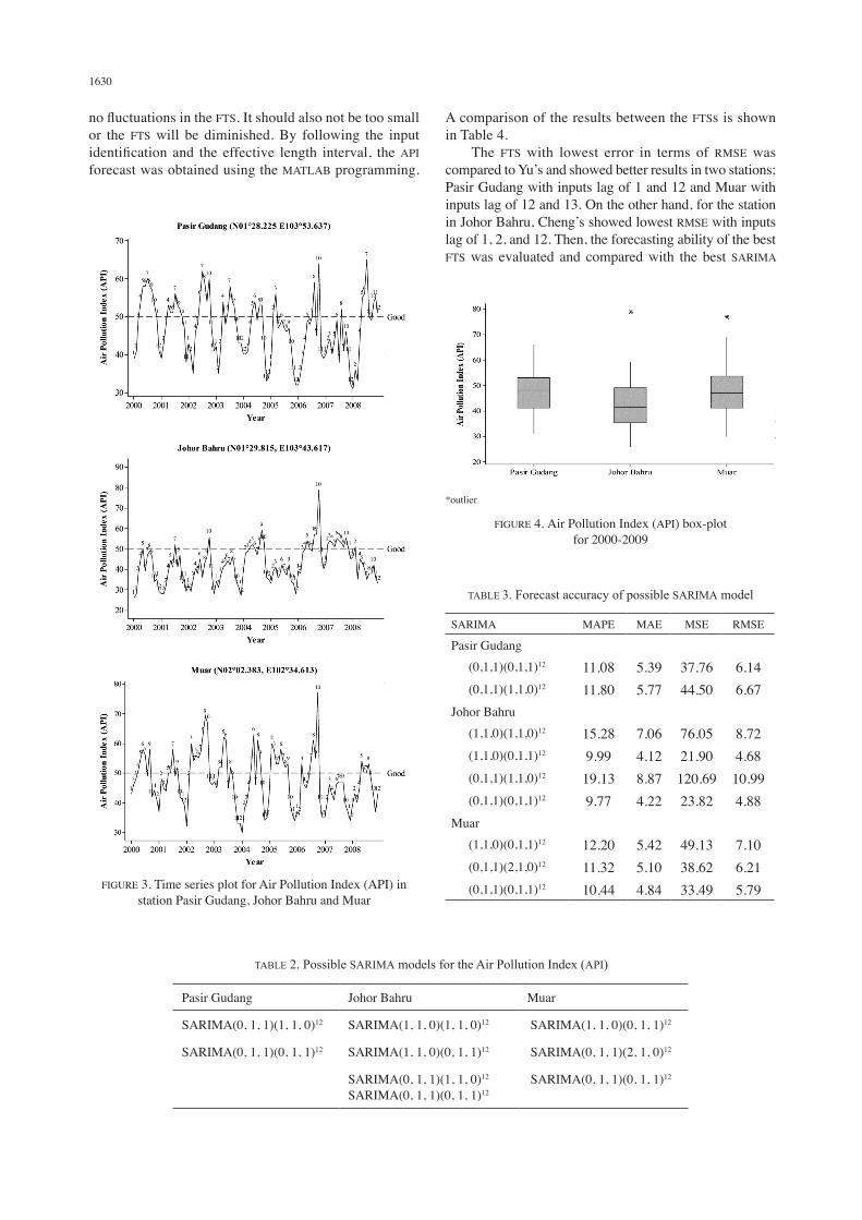
monitoring stations in the Malaysian Peninsular are affected by the transboundary sources of biomass burning around Southeast Asia, especially from Sumatra, Indonesia (Nurulilyana et al. 2011). Therefore, in the box plot, the outlier was detected at two stations, Johor Bahru and Muar as presented in Figure 4. The descriptive statistics of monthly mean API showed that the highest values were recorded in Muar, followed by Pasir Gudang and Johor Bahru. These findings demonstrate that the API correlates with PM10 and O3 trends. Moreover, the result verifies the DoE annual report (2011) which states that PM10 and O3 are the predominant pollutants causing unhealthy air quality status for several years. The time series plot gives important information for the determination of the trend and seasonality of the data set before ascertaining the tentative model identification. The details of seasonal variations of API, based on the profiles, are shown in Figure 3. The existence of a seasonal pattern indicates that the data is non-stationary either in mean or variance. However, based on the box-cox plot, the API data spread within the constant level over time in variance, indicating the data was stationary in variance but not in mean. By taking the difference d = 1 for non-seasonal and D = 1 with S =12 for the seasonal part, the data becomes a stationary series. By following this, the tentative model for autocorrelation function (ACF) and partial autocorrelation function (PACF) were used to determine the best combination order of ARIMA model as shown in Table 2.

TABLE 1. Descriptive statistics on air quality data at the different stations in Johor

Parameters Station Average Median S.D. Minimum Maximum RMAQG

PM10 (μgm-3)

Pasir Gudang 49.86 49.98 10.56 30.32 83.76 150Johor Bahru 42.12 39.01 12.03 23.05 109.14Muar 51.61 49.78 13.81 29.77 105.56

CO (ppm)

Pasir Gudang 0.689 0.682 0.151 0.374 1.173 30Johor Bahru 0.626 0.631 0.175 0.282 1.079Muar 0.541 0.517 0.141 0.305 1.186

NO2 (ppm)

Pasir Gudang 0.013 0.014 0.004 0.005 0.031 0.17Johor Bahru 0.015 0.016 0.004 0.008 0.023Muar 0.009 0.008 0.002 0.004 0.013

SO2 (ppm)

Pasir Gudang 0.007 0.006 0.005 0.001 0.022 0.13Johor Bahru 0.007 0.007 0.004 0.001 0.020Muar 0.002 0.002 0.001 0.000 0.004

O3 (ppm)

Pasir Gudang 0.013 0.013 0.003 0.008 0.023 0.10Johor Bahru 0.014 0.014 0.002 0.009 0.021Muar 0.019 0.018 0.003 0.007 0.029

API Pasir Gudang 47.51 48.00 7.98 31 66 50Johor Bahru 42.18 41.50 8.77 26 79Muar 47.65 47.00 8.78 30 77

RMAQG = Recommended Malaysian Air Quality Guidelines

1629

The significant model can be determined using the Ljung-Box test and checking the p-value of the coefficient. Out of all possibilities of the SARIMA model, the best combination model was chosen based on the smallest RMSE. Based on Table 3, the best model to describe the API trends in Pasir Gudang and Muar is SARIMA (0,1,1)(0,1,1)12 can be written as:

yt = yt-1 +yt-12 – yt-13 + εt – θεt-1 – Θεt-12 + Θθεt-13.

For station in Johor Bahru SARIMA (1,1,0)(0,1,1)12. Thus, the model equation is:

yt = yt-1 +nyt-12 – yt-13 + ϕyt-1 – ϕyt-2 – ϕyt-13 – ϕyt-14

+ εt – Θθεt-12.

For the second statistical model, the FTS method discussed previously, all of the computations for FTS (i.e. Chen’s, Yu’s, Cheng’s) were performed using MATLAB software. In FTS, it is crucial to identify the best input to achieve the required FLR for a better forecasting result. Generally, the input selection used in the FTS is obtained from the ARIMA model. For the stations in Pasir Gudang and Muar, the FLR could be up to three input lags (lag 1, 12 and 13), whereas for the station in Johor Bahru, the FLR there could be up to five input lags (lag 1, 2, 12, 13 and 14). Besides determining the input, the length of intervals also affects the performance of forecasting results in FTS because different lengths may lead to a range of forecasting results. According to Huarng (2001), the effective length should not to be too large or there will be

FIGURE 2. Monthly trends of air quality in Johor (2000-2009)

1630

FIGURE 3. Time series plot for Air Pollution Index (API) in station Pasir Gudang, Johor Bahru and Muar

*outlier

FIGURE 4. Air Pollution Index (API) box-plot for 2000-2009

TABLE 2. Possible SARIMA models for the Air Pollution Index (API)

Pasir Gudang Johor Bahru Muar

SARIMA(0, 1, 1)(1, 1, 0)12 SARIMA(1, 1, 0)(1, 1, 0)12 SARIMA(1, 1, 0)(0, 1, 1)12

SARIMA(0, 1, 1)(0, 1, 1)12 SARIMA(1, 1, 0)(0, 1, 1)12 SARIMA(0, 1, 1)(2, 1, 0)12

SARIMA(0, 1, 1)(1, 1, 0)12

SARIMA(0, 1, 1)(0, 1, 1)12 SARIMA(0, 1, 1)(0, 1, 1)12

TABLE 3. Forecast accuracy of possible SARIMA model

SARIMA MAPE MAE MSE RMSE

Pasir Gudang (0,1,1)(0,1,1)12 11.08 5.39 37.76 6.14 (0,1,1)(1,1,0)12 11.80 5.77 44.50 6.67Johor Bahru (1,1,0)(1,1,0)12 15.28 7.06 76.05 8.72 (1,1,0)(0,1,1)12 9.99 4.12 21.90 4.68 (0,1,1)(1,1,0)12 19.13 8.87 120.69 10.99 (0,1,1)(0,1,1)12 9.77 4.22 23.82 4.88Muar (1,1,0)(0,1,1)12 12.20 5.42 49.13 7.10 (0,1,1)(2,1,0)12 11.32 5.10 38.62 6.21 (0,1,1)(0,1,1)12 10.44 4.84 33.49 5.79

no fluctuations in the FTS. It should also not be too small or the FTS will be diminished. By following the input identification and the effective length interval, the API forecast was obtained using the MATLAB programming.

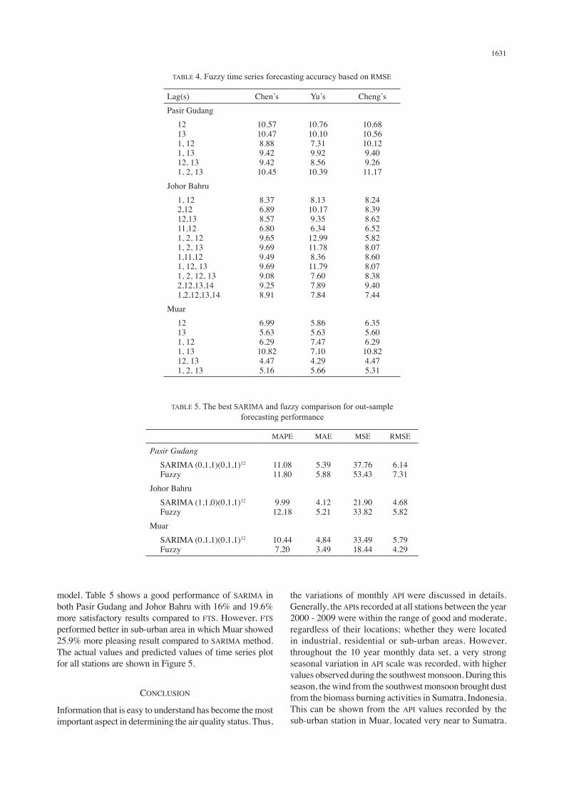
A comparison of the results between the FTSs is shown in Table 4. The FTS with lowest error in terms of RMSE was compared to Yu’s and showed better results in two stations; Pasir Gudang with inputs lag of 1 and 12 and Muar with inputs lag of 12 and 13. On the other hand, for the station in Johor Bahru, Cheng’s showed lowest RMSE with inputs lag of 1, 2, and 12. Then, the forecasting ability of the best FTS was evaluated and compared with the best SARIMA

1631

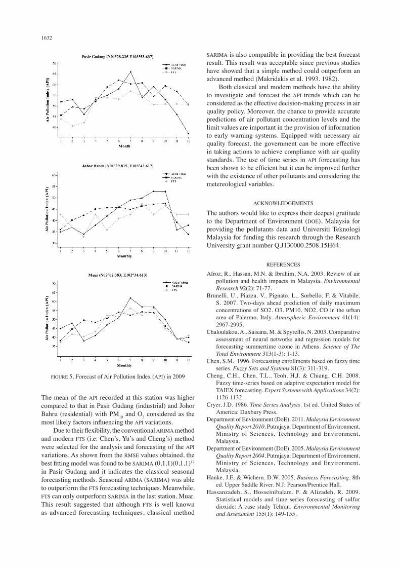
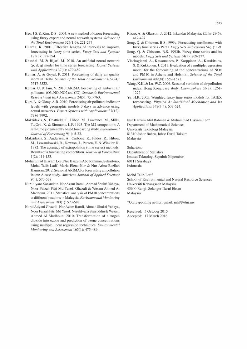
model. Table 5 shows a good performance of SARIMA in both Pasir Gudang and Johor Bahru with 16% and 19.6% more satisfactory results compared to FTS. However, FTS performed better in sub-urban area in which Muar showed 25.9% more pleasing result compared to SARIMA method. The actual values and predicted values of time series plot for all stations are shown in Figure 5.

CONCLUSION

Information that is easy to understand has become the most important aspect in determining the air quality status. Thus,

the variations of monthly API were discussed in details. Generally, the APIs recorded at all stations between the year 2000 - 2009 were within the range of good and moderate, regardless of their locations; whether they were located in industrial, residential or sub-urban areas. However, throughout the 10 year monthly data set, a very strong seasonal variation in API scale was recorded, with higher values observed during the southwest monsoon. During this season, the wind from the southwest monsoon brought dust from the biomass burning activities in Sumatra, Indonesia. This can be shown from the API values recorded by the sub-urban station in Muar, located very near to Sumatra.

TABLE 4. Fuzzy time series forecasting accuracy based on RMSE

Lag(s) Chen’s Yu’s Cheng’sPasir Gudang 12 13 1, 12 1, 13 12, 13 1, 2, 13

10.5710.478.889.429.4210.45

10.7610.107.319.928.5610.39

10.6810.5610.129.409.2611.17

Johor Bahru 1, 12 2,12 12,13 11,12 1, 2, 12 1, 2, 13 1,11,12 1, 12, 13 1, 2, 12, 13 2,12,13,14 1,2,12,13,14

8.376.898.576.809.659.699.499.699.089.258.91

8.1310.179.356.3412.9911.788.3611.797.607.897.84

8.248.398.626.525.828.078.608.078.389.407.44

Muar 12 13 1, 12 1, 13 12, 13 1, 2, 13

6.995.636.2910.824.475.16

5.865.637.477.104.295.66

6.355.606.2910.824.475.31

TABLE 5. The best SARIMA and fuzzy comparison for out-sample forecasting performance

MAPE MAE MSE RMSE

Pasir Gudang

SARIMA (0,1,1)(0,1,1)12

Fuzzy 11.0811.80

5.395.88

37.7653.43

6.147.31

Johor Bahru SARIMA (1,1,0)(0,1,1)12

Fuzzy9.9912.18

4.125.21

21.9033.82

4.685.82

Muar SARIMA (0,1,1)(0,1,1)12

Fuzzy10.447.20

4.843.49

33.4918.44

5.794.29

1632

The mean of the API recorded at this station was higher compared to that in Pasir Gudang (industrial) and Johor Bahru (residential) with PM10 and O3 considered as the most likely factors influencing the API variations. Due to their flexibility, the conventional ARIMA method and modern FTS (i.e: Chen’s, Yu’s and Cheng’s) method were selected for the analysis and forecasting of the API variations. As shown from the RMSE values obtained, the best fitting model was found to be SARIMA (0,1,1)(0,1,1)12 in Pasir Gudang and it indicates the classical seasonal forecasting methods. Seasonal ARIMA (SARIMA) was able to outperform the FTS forecasting techniques. Meanwhile, FTS can only outperform SARIMA in the last station, Muar. This result suggested that although FTS is well known as advanced forecasting techniques, classical method

SARIMA is also compatible in providing the best forecast result. This result was acceptable since previous studies have showed that a simple method could outperform an advanced method (Makridakis et al. 1993, 1982). Both classical and modern methods have the ability to investigate and forecast the API trends which can be considered as the effective decision-making process in air quality policy. Moreover, the chance to provide accurate predictions of air pollutant concentration levels and the limit values are important in the provision of information to early warning systems. Equipped with necessary air quality forecast, the government can be more effective in taking actions to achieve compliance with air quality standards. The use of time series in API forecasting has been shown to be efficient but it can be improved further with the existence of other pollutants and considering the metereological variables.

ACKNOWLEDGEMENTS

The authors would like to express their deepest gratitude to the Department of Environment (DOE), Malaysia for providing the pollutants data and Universiti Teknologi Malaysia for funding this research through the Research University grant number Q.J130000.2508.15H64.

REFERENCES

Afroz, R., Hassan, M.N. & Ibrahim, N.A. 2003. Review of air pollution and health impacts in Malaysia. Environmental Research 92(2): 71-77.

Brunelli, U., Piazza, V., Pignato, L., Sorbello, F. & Vitabile, S. 2007. Two-days ahead prediction of daily maximum concentrations of SO2, O3, PM10, NO2, CO in the urban area of Palermo, Italy. Atmospheric Environment 41(14): 2967-2995.

Chaloulakou, A., Saisana, M. & Spyrellis, N. 2003. Comparative assessment of neural networks and regression models for forecasting summertime ozone in Athens. Science of The Total Environment 313(1-3): 1-13.

Chen, S.M. 1996. Forecasting enrollments based on fuzzy time series. Fuzzy Sets and Systems 81(3): 311-319.

Cheng, C.H., Chen, T.L., Teoh, H.J. & Chiang, C.H. 2008. Fuzzy time-series based on adaptive expectation model for TAIEX forecasting. Expert Systems with Applications 34(2): 1126-1132.

Cryer, J.D. 1986. Time Series Analysis. 1st ed. United States of America: Duxbury Press.

Department of Environment (DoE). 2011. Malaysia Environment Quality Report 2010. Putrajaya: Department of Environment, Ministry of Sciences, Technology and Environment, Malaysia.

Department of Environment (DoE). 2005. Malaysia Environment Quality Report 2004. Putrajaya: Department of Environment, Ministry of Sciences, Technology and Environment, Malaysia.

Hanke, J.E. & Wichern, D.W. 2005. Business Forecasting. 8th ed. Upper Saddle River, N.J: Pearson/Prentice Hall.

Hassanzadeh, S., Hosseinibalam, F. & Alizadeh, R. 2009. Statistical models and time series forecasting of sulfur dioxide: A case study Tehran. Environmental Monitoring and Assessment 155(1): 149-155.

FIGURE 5. Forecast of Air Pollution Index (API) in 2009

1633

Heo, J.S. & Kim, D.S. 2004. A new method of ozone forecasting using fuzzy expert and neural network systems. Science of the Total Environment 325(1-3): 221-237.

Huarng, K. 2001. Effective lengths of intervals to improve forecasting in fuzzy time series. Fuzzy Sets and Systems 123(3): 387-394.

Khashei, M. & Bijari, M. 2010. An artificial neural network (p, d, q) model for time series forecasting. Expert Systems with Applications 37(1): 479-489.

Kumar, A. & Goyal, P. 2011. Forecasting of daily air quality index in Delhi. Science of the Total Environment 409(24): 5517-5523.

Kumar, U. & Jain, V. 2010. ARIMA forecasting of ambient air pollutants (O3, NO, NO2 and CO). Stochastic Environmental Research and Risk Assessment 24(5): 751-760.

Kurt, A. & Oktay, A.B. 2010. Forecasting air pollutant indicator levels with geographic models 3 days in advance using neural networks. Expert Systems with Applications 37(12): 7986-7992.

Makridakis, S., Chatfield, C., Hibon, M., Lawrence, M., Mills, T., Ord, K. & Simmons, L.F. 1993. The M2-competition: A real-time judgmentally based forecasting study. International Journal of Forecasting 9(1): 5-22.

Makridakis, S., Andersen, A., Carbone, R., Fildes, R., Hibon, M., Lewandowski, R., Newton, J., Parzen, E. & Winkler, R. 1982. The accuracy of extrapolation (time series) methods: Results of a forecasting competition. Journal of Forecasting 1(2): 111-153.

Muhammad Hisyam Lee, Nur Haizum Abd Rahman, Suhartono, Mohd Talib Latif, Maria Elena Nor & Nur Arina Bazilah Kamisan. 2012. Seasonal ARIMA for forecasting air pollution index: A case study. American Journal of Applied Sciences 9(4): 570-578.

Nurulilyana Sansuddin, Nor Azam Ramli, Ahmad Shukri Yahaya, Noor Faizah Fitri Md Yusof, Ghazali & Wesam Ahmed Al Madhoun. 2011. Statistical analysis of PM10 concentrations at different locations in Malaysia. Environmental Monitoring and Assessment 180(1): 573-588.

Nurul Adyani Ghazali, Nor Azam Ramli, Ahmad Shukri Yahaya, Noor Faizah Fitri Md Yusof, Nurulilyana Sansuddin & Wesam Ahmed Al Madhoun. 2010. Transformation of nitrogen dioxide into ozone and prediction of ozone concentrations using multiple linear regression techniques. Environmental Monitoring and Assessment 165(1): 475-489.

Rizzo, A. & Glasson, J. 2012. Iskandar Malaysia. Cities 29(6): 417-427.

Song, Q. & Chissom, B.S. 1993a. Forecasting enrollments with fuzzy time series - Part I. Fuzzy Sets and Systems 54(1): 1-9.

Song, Q. & Chissom, B.S. 1993b. Fuzzy time series and its models. Fuzzy Sets and Systems 54(3): 269-277.

Vlachogianni, A., Kassomenos, P., Karppinen, A., Karakitsios, S. & Kukkonen, J. 2011. Evaluation of a multiple regression model for the forecasting of the concentrations of NOx and PM10 in Athens and Helsinki. Science of the Total Environment 409(8): 1559-1571.

Wang, X.K. & Lu, W.Z. 2006. Seasonal variation of air pollution index: Hong Kong case study. Chemosphere 63(8): 1261-1272.

Yu, H.K. 2005. Weighted fuzzy time series models for TAIEX forecasting. Physica A: Statistical Mechanics and Its Applications 349(3-4): 609-624.

Nur Haizum Abd Rahman & Muhammad Hisyam Lee*Department of Mathematical Sciences Universiti Teknologi Malaysia 81310 Johor Bahru, Johor Darul Takzim Malaysia

SuhartonoDepartment of Statistics Institut Teknologi Sepuluh Nopember 60111 SurabayaIndonesia

Mohd Talib LatifSchool of Environmental and Natural Resource Sciences Universiti Kebangsaan Malaysia43600 Bangi, Selangor Darul Ehsan Malaysia

*Corresponding author; email: mhl@utm.my

Received: 5 October 2015Accepted: 17 March 2016