
VOT 74204 DEVELOPMENT OF A SEMI-SWATH CRAFT FOR … · Kesahan nialaian menggunanakan persamaan...
246
VOT 74204 DEVELOPMENT OF A SEMI-SWATH CRAFT FOR MALAYSIAN WATERS (PEMBANGUNAN KAPAL SEMI-SWATH UNTUK PERAIRAN MALAYSIA) OMAR BIN YAAKOB FAKULTI KEJURUTERAAN MEKANIKAL UNIVERSITI TEKNOLOGI MALAYSIA 2006
Transcript of VOT 74204 DEVELOPMENT OF A SEMI-SWATH CRAFT FOR … · Kesahan nialaian menggunanakan persamaan...
VOT 74204
DEVELOPMENT OF A SEMI-SWATH CRAFT FOR MALAYSIAN WATERS
(PEMBANGUNAN KAPAL SEMI-SWATH UNTUK PERAIRAN MALAYSIA)
OMAR BIN YAAKOB
FAKULTI KEJURUTERAAN MEKANIKAL
UNIVERSITI TEKNOLOGI MALAYSIA
2006
VOT 74204
DEVELOPMENT OF A SEMI-SWATH CRAFT FOR MALAYSIAN WATERS
(PEMBANGUNAN KAPAL SEMI-SWATH UNTUK PERAIRAN MALAYSIA)
OMAR BIN YAAKOB
RESEARCH VOTE NO:
74204
FAKULTI KEJURUTERAAN MEKANIKAL
UNIVERSITI TEKNOLOGI MALAYSIA
2006

ii
ACKNOWLEDGEMENT
The researchers wish to thank MOSTI who supported the project under the
IRPA programme. Staff at Research Management Centre UTM have been very
helpful and for that we are very grateful. We also wish to record our gratitude to
friends and staff of Marine Technology Laboratory and the Composite Cente for
their support is the construction and testing of the model and prototype.
iii
ABSTRACT
Small Waterplane Area Twin Hull (SWATH) and Catamaran vessels are known to
have more stable platform as compared to mono-hulls. A further advantage of
SWATH as compared to Catamaran is its smaller waterplane area that provides
better seakeeping qualities. However, the significant drawback of the SWATH vessel
is when encountering head-sea at high forward speed. Due to its low stiffness, it has
a tendency for large pitch motions. Consequently, this may lead to excessive trim or
even deck wetness. This phenomenon will not only degrade the comfortability but
also results in structural damage with greater safety risks. In this research a modified
SWATH design is proposed. The proposed design concept represents a combination
of Catamaran and SWATH vessel hull features that will lead to reduce in bow-diving
but still maintains good seakeeping capabilities. This is then called the Semi-
SWATH vessel. In addition, the full-design of this vessel has been equipped by fixed
fore fins and controllable aft fins attached on each lower hull. In the development of
controllable aft fins, the PID controller system was applied to obtain an optimal
vessel’s ride performance at speeds of 15 (medium) and 20 (high) knots.
In this research work, the seakeeping performance of Semi-SWATH vessel was
evaluated using time-domain simulation approach. The effect of fin stabilizer on the
bare hull performance is considered. The validity of numerical evaluation was then
compared with model experiments carried out in the Towing Tank at Marine
Technology Laboratory, UTM. It is shown that the Semi-SWATH vessel with
controllable fin stabilizer can have significantly reduction by about 42.57% of heave
motion and 48.80% of pitch motion.
Key researchers : Prof. Madya Dr. Omar Bin Yaakob (Head)
Prof. Madya Dr. Adi Maimun Bin Haji Abdul Malik Haji Yahya Bin Samian
Ahmad Fitriadhy
E-mail : [email protected] Tel. No. : 07-5535700
Vote No. : 74204
iv
ABSTRAK
Adalah diketahui bahawa Small Waterplane Area Twin Hull (SWATH) dan
Catamaran mempunyai pelantar yang lebih stabil dibandingkan dengan mono-hull.
Kelebihan SWATH adalah kawasan ‘waterplane’ yang lebih kecil untuk
menghasilkan kualiti pergerakan kapal yang lebih baik berbanding Catamaran.
Walaubagaimanapun, kekurangan SWATH adalah apabila menempuh laut pada
kelajuan yang tinggi. Berdasarkan pada tahap kekerasan kapal ini yang rendah, kapal
ini cenderung megalami pergerakan picth yang besar. Ini akan mengakibatkan trim
yang berlebihan atau kebasahan dek. Fenomena ini bukan sahaja mengurangkan
keselesaan tetapi juga menyebabkan kerosakan stuktur dengan risiko keselamatan
yang lebih tingi. Penyelidikan ini mencadangkan rekabentuk SWATH yang
diubahsuai. Konsep rekabentuk yang dicadangkan menunjukkan kombinasi ciri-ciri
badan kapal Catamaran dan SWATH yang akan mengurangkan ‘bow-diving’ tetapi
masih mengekalkan kebolehan pergerakan yang baik. Ini dikenali sebagai Semi-
SWATH. Tambahan pula rekabentuk lengkap bagi kapal ini dilengkapi dengan sirip
tetap dibahagian depan dan sirip bolehkawal dibahagian belakang pada setiap badan
kapal yang lebih rendah. Dalam membangunkan sirip bolehkawal dibahagian
belakang kapal, sistem pengawal PID telah digunakan untuk mendapatkan keadaan
perjalanan kapal yang optimum pada kelajuan 15 (sederhana) dan 20 (tinggi) knots.
Dalam kerje penyelidikan ini, pergerakan Semi-SWATH telah dinilai menggunakan
kaedah simulasi domain-masa. Kesan pemantap sirip pada badan kapal yang kosong
dipertimbangkan. Kesahan nialaian menggunanakan persamaan matematik
dibandingkan dengan eksperimen model yang telah dilakukan dalam Tangki Tunda
di Makmal Teknologi Marin, UTM. Ini menunjukkan Semi-SWATH dengan
pemantap sirip bolehkawal mempunyai pengurangan sebanyak 42.57% bagi
pergerakan heave dan 48.80% bagi pergerakan pitch.
Key researchers : Prof. Madya Dr. Omar Bin Yaakob (Head)
Prof. Madya Dr. Adi Maimun Bin Haji Abdul Malik Haji Yahya Bin Samian
Ahmad Fitriadhy E-mail : [email protected]
Tel. No. : 07-5535700 Vote No. : 74204

v
TABLE OF CONTENTS
CHAPTER TITLE PAGE
ACKNOWLEGDEMENT ii
ABSTRACT iii
ABSTRAK iv
TABLE OF CONTENTS v
LIST OF TABLES x
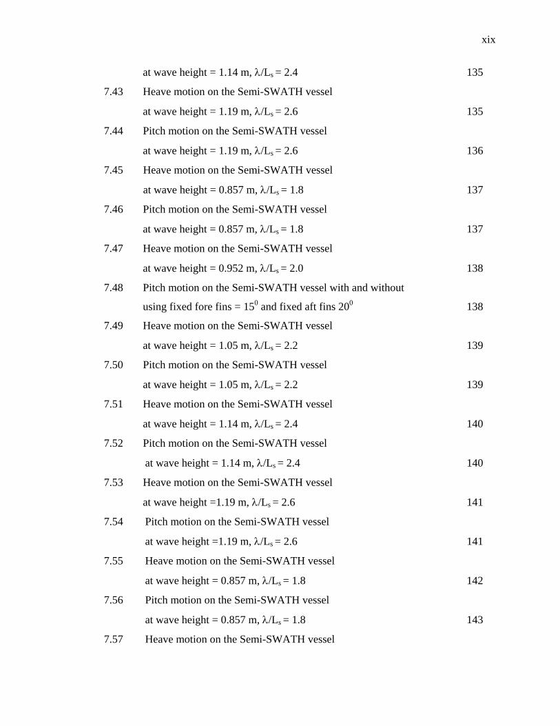
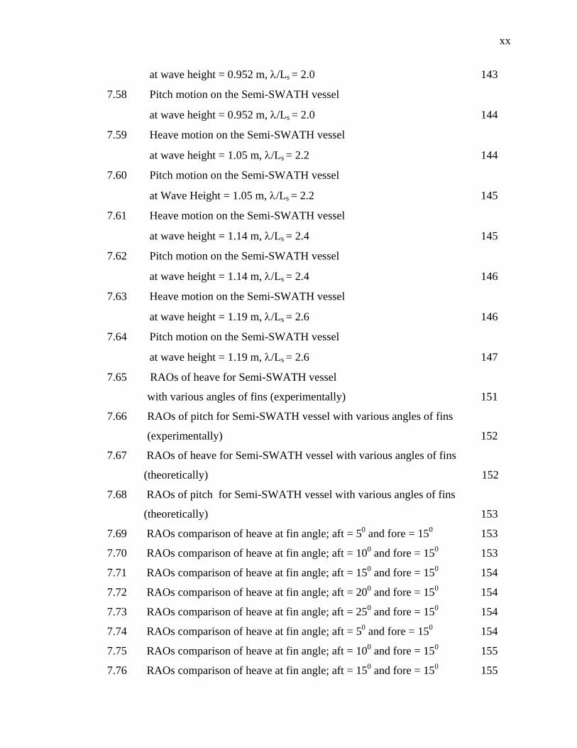
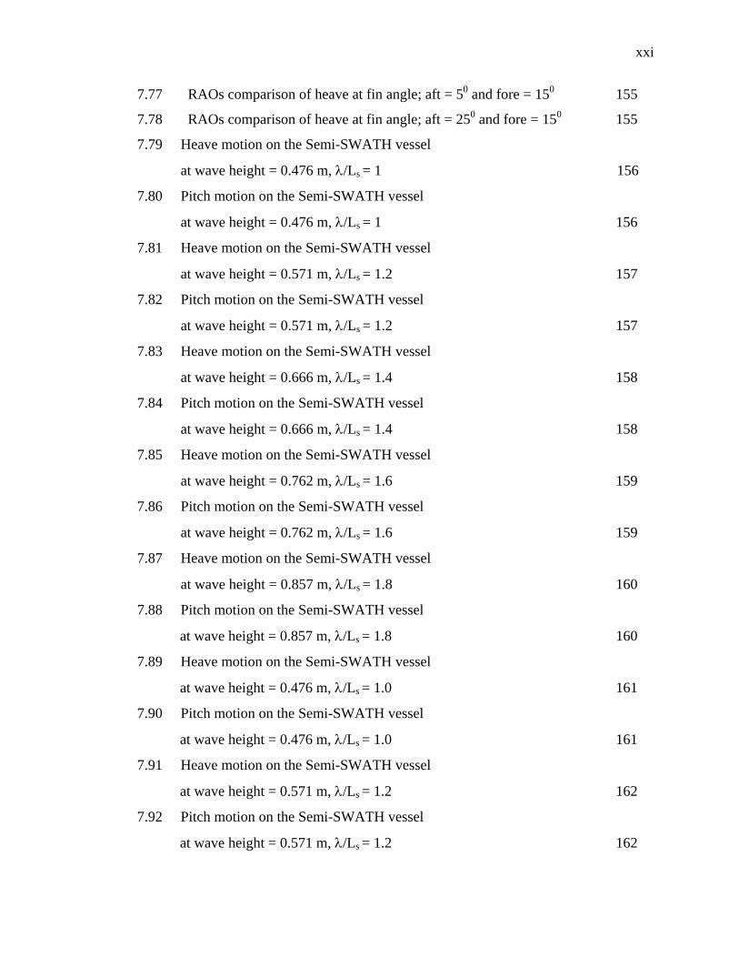
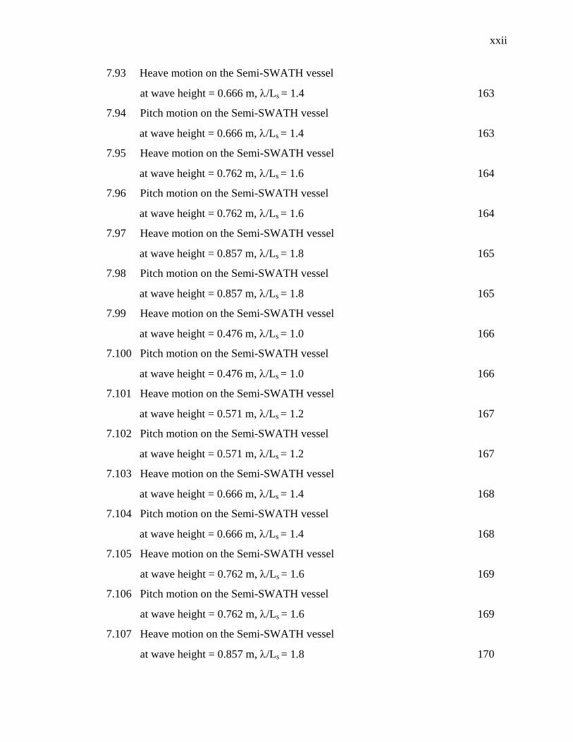
LIST OF FIGURES xiii
NOMENCLATURE xxv
LIST OF APPENDICES xxx
1 INTRODUCTION 1
1.1 Background 1
1.2 Research Objective 3
1.3 Scope of Research 4
1.4 Research Outline 5
2 LITERATURE REVIEW 7
2.1 General 7
2.2 Historical Design of Semi-SWATH vessel 8
2.2.1 Catamaran 8
2.2.1.1 The advantages of Catamaran 9
2.2.1.2 The drawback of Catamaran 10
2.2.3 SWATH vessel 11
2.2.3.1 The advantages of SWATH vessel 11
vi
2.2.3.2 The drawback of SWATH vessel 12
2.3 The Concept of the Semi-SWATH vessel 14
2.3.1 Advantages of Semi-SWATH vessel 15
2.3.2 Motion Response of Semi-SWATH vessel 16
2.4 Prediction of Ship Motion 18
2.5 Motion Characteristics of High-Speed Twin-Hull Vessel 21
2.6 The Effect of Heave and Pitch Motion Responses 21
2.7 Pitch Motion Stabilizations 23
2.7.1 Fixed Bow Fin 26
2.7.2 Controllable Stern Fin 27
2.7.3 Design of Fin 29
2.8 Ride-Control System 31
2.8.1 Application of PID Controller on
The Ship Motion Improvement 32
2.9 Time-Domain Simulation 34
2.10 Seakeeping Assessment 36
3 APPROACH 37
3.1 General 37
3.2 Framework of Study 38
3.3 Choosing a Systematic Procedure 41
3.3.1 Selection of Parameters 42
3.3.2 Parametric Study 43
3.3.3 Evaluation of Motion Response 45
3.4 Concluding Remarks 45
4 MATHEMATICAL MODEL 46
4.1 General 46
4.2 Formulation of Hydrodynamic Forces and Moments
Based On Strip Theory 47
4.2.1 Co-ordinate System 47
4.2.2 Boundary Conditions and Linearization 48
vii
4.2.3 Application of Strip Theory 52
4.2.4 Hydrodynamic Forces and Moments 55
4.3 Modelling of Fin Effect 56
4.4 Equations of Motion in Time-Domain Simulation 66
4.4.1 Solution of The Motion Equations 69
4.5 Concluding Remarks 69
5 IMPROVED VESSEL RIDE PERFORMANCE
USING TIME-DOMAIN SIMULATION 69
5.1 General 69
5.2 Simple Block of Control System using PID Controller 70
5.3 The Three-Term PID Controller 70
5.4 The Proportional-Integral-Derivative (PID) algorithm 71
5.4.1 A Proportional Algorithm 73
5.4.2 A Proportional Integral Algorithm 72
5.4.3 A Proportional Integral Derivative Algorithm 72
5.5 Controller Tuning 73
5.5.1 Parameter Tuning Rules for PID Controller 73
5.6 Actuator Modeling 75
5.6.1 Modeling of DC Servomotor 75
5.7 Application of PID Controller to Multi-Hull Motion Control 79
5.8 Closed-Loop of Anti-Pitching Fin Control System 80
5.9 Time-Domain Simulation Program Structure 81
5.10 Computer Simulation 82
5.11 Simulation Condition 83
5.12 Simulation Results 84
5.12.1 First Simulation Results 85
5.12.2 Second Simulation Results 91
5.13 Concluding Remarks 96
viii
6 PROCEDURE OF SEAKEEPING TEST 98
6.1 General 98
6.2 Objective of The Experiments 98
6.3 Model Test Preparation 99
6.3.1 Model Test Particulars 100
6.4 Experiments Apparatus and Facility 102
6.4.1 Towing Tank 102
6.4.2 Towing Carriage 103
6.4.3 Wave Generator 103
6.5 Experiments Setup 103
6.6 Experiment Condition 106
6.7 Description of Data Test Analysis 106
6.8 Concluding Remarks 107
7 VALIDATION 109
7.1 General 109
7.2 Comparison of Experimental and Simulation Results 109
7.3 Case 1 112
7.3.1 Maximum and Minimum Values of Heave
and Pitch Motion at T=2.0m and Vs=15 Knots 112
7.3.2 Response Amplitude Operators (RAOs)
of Heave and Pitch Motion T=2.0m and Vs=15 Knots 114
7.3.3 Time-Histories of Heave and Pitch Motion
T=2.0m and Vs=15 Knots 120
7.4 Case 2 147
7.4.1 Maximum and Minimum Values of Heave and Pitch Motion
at T=1.4 m and Vs=20 Knots 147
7.4.2 Response Amplitude Operators (RAOs)
of Heave and Pitch Motion T=1.4 m and Vs=20 Knots 149
7.4.3 Time-Histories of Heave and Pitch Motion
T=1.4 m and Vs=20 Knots 155
7.5 Concluding Remarks 180
ix
8 DISCUSSION 181
8.1 General 181
8.2 Mathematical model 183
8.3 Investigation of Controller Scheme of The Fin Stabilizers 183
8.4 Development of PID Controller 185
8.5 Experimental Result 185
8.6 Concluding Remarks 186
9 CONCLUSSION 187
10 FUTURE RESEARCH 189
REFERENCES 190
APPENDICES
APPENDIX A 199
APPENDIX B 204
APPENDIX C 206
APPENDIX D 209
APPENDIX E 211
APPENDIX F 213
x
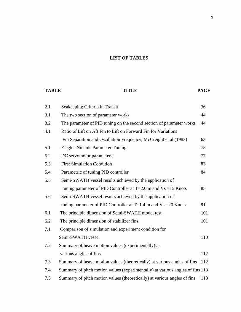
LIST OF TABLES
TABLE TITLE PAGE
2.1 Seakeeping Criteria in Transit 36
3.1 The two section of parameter works 44
3.2 The parameter of PID tuning on the second section of parameter works 44
4.1 Ratio of Lift on Aft Fin to Lift on Forward Fin for Variations
Fin Separation and Oscillation Frequency, McCreight et al (1983) 63
5.1 Ziegler-Nichols Parameter Tuning 75
5.2 DC servomotor parameters 77
5.3 First Simulation Condition 83
5.4 Parametric of tuning PID controller 84
5.5 Semi-SWATH vessel results achieved by the application of
tuning parameter of PID Controller at T=2.0 m and Vs =15 Knots 85
5.6 Semi-SWATH vessel results achieved by the application of
tuning parameter of PID Controller at T=1.4 m and Vs =20 Knots 91
6.1 The principle dimension of Semi-SWATH model test 101
6.2 The principle dimension of stabilizer fins 101
7.1 Comparison of simulation and experiment condition for
Semi-SWATH vessel 110
7.2 Summary of heave motion values (experimentally) at
various angles of fins 112
7.3 Summary of heave motion values (theoretically) at various angles of fins 112
7.4 Summary of pitch motion values (experimentally) at various angles of fins 113
7.5 Summary of pitch motion values (theoretically) at various angles of fins 113
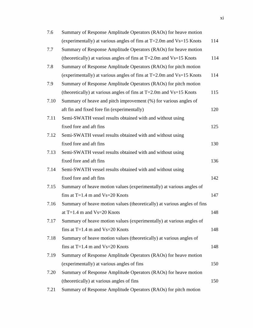
xi
7.6 Summary of Response Amplitude Operators (RAOs) for heave motion
(experimentally) at various angles of fins at T=2.0m and Vs=15 Knots 114
7.7 Summary of Response Amplitude Operators (RAOs) for heave motion
(theoretically) at various angles of fins at T=2.0m and Vs=15 Knots 114
7.8 Summary of Response Amplitude Operators (RAOs) for pitch motion
(experimentally) at various angles of fins at T=2.0m and Vs=15 Knots 114
7.9 Summary of Response Amplitude Operators (RAOs) for pitch motion
(theoretically) at various angles of fins at T=2.0m and Vs=15 Knots 115
7.10 Summary of heave and pitch improvement (%) for various angles of
aft fin and fixed fore fin (experimentally) 120
7.11 Semi-SWATH vessel results obtained with and without using
fixed fore and aft fins 125
7.12 Semi-SWATH vessel results obtained with and without using
fixed fore and aft fins 130
7.13 Semi-SWATH vessel results obtained with and without using
fixed fore and aft fins 136
7.14 Semi-SWATH vessel results obtained with and without using
fixed fore and aft fins 142
7.15 Summary of heave motion values (experimentally) at various angles of
fins at T=1.4 m and Vs=20 Knots 147
7.16 Summary of heave motion values (theoretically) at various angles of fins
at T=1.4 m and Vs=20 Knots 148
7.17 Summary of heave motion values (experimentally) at various angles of
fins at T=1.4 m and Vs=20 Knots 148
7.18 Summary of heave motion values (theoretically) at various angles of
fins at T=1.4 m and Vs=20 Knots 148
7.19 Summary of Response Amplitude Operators (RAOs) for heave motion
(experimentally) at various angles of fins 150
7.20 Summary of Response Amplitude Operators (RAOs) for heave motion
(theoretically) at various angles of fins 150
7.21 Summary of Response Amplitude Operators (RAOs) for pitch motion
xii
(experimentally) at various angles of fins 150
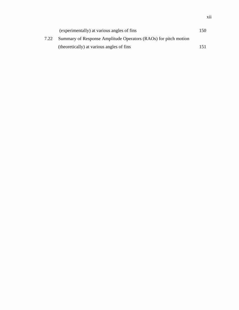
7.22 Summary of Response Amplitude Operators (RAOs) for pitch motion
(theoretically) at various angles of fins 151

xiii
LIST OF FIGURES
FIGURE TITLE PAGE
1.1 Outline of the thesis organization 6
2.1 Catamaran vessel profile and section 9
2.2 Conventional SWATH vessel profile and section 11
2.3 Illustration of strip theory for ships, Faltinsen (1990) 18
4.1 Definition of vessel’s coefficient-ordinate system 48
4.2 Description of defined boundaries fluid for twin-hull vessels 52
4.3 Comparison of Wing-Body interaction Factors for Fixed Fin (Caldeira-
Saraiva and Clarke, 1988) 58
4.4 Comparison of Wing-Body interaction Factors for Movable Fins
(Caldeira-Saraiva and Clarke, 1988) 59
4.5 Effect of Boundary Layer on Fin Lift, Lloyd (1989) 60
4.6 Trailing Vortex Generated by a Lifting Surface, Lloyd, (1989) 61
4.7 Fin-Fin Interference for Oscillating Fins, Lloyd, (1989) 61
4.8 Fin-Fin Interference Factors, Lloyd, (1989) 62
4.9 Variation of Lift with Submergence, Atlar, Kenevissi et al (1997) 63
4.10 Representation of The Geometric Parameters for Hull-Fin Interference
Atlar (1991) 64
4.11 The Drag Coefficient of Flat Plate (+), Diamond (◊) and Circular (o)
Cylinders at Low KC, Bearman, et al (1979) 65
5.1 Simple Block of Control System 70
xiv
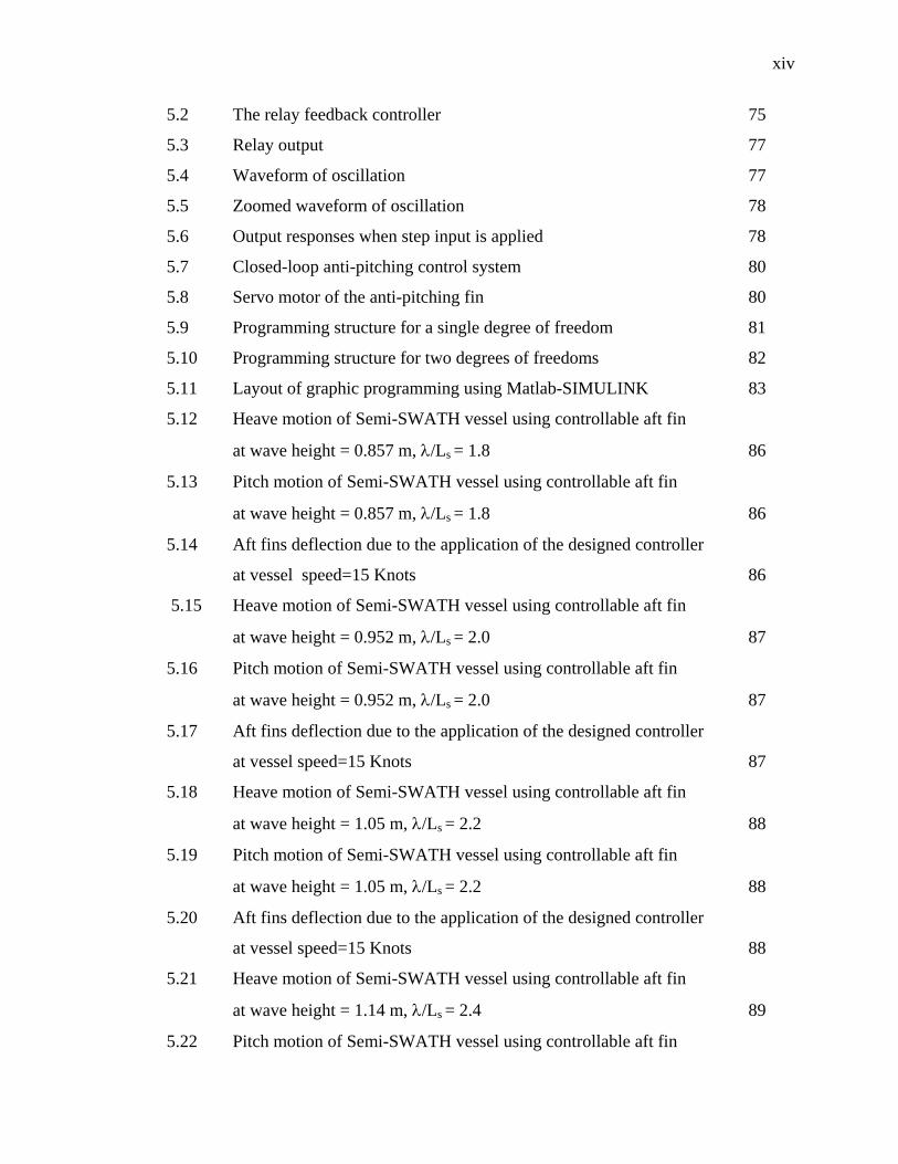
5.2 The relay feedback controller 75
5.3 Relay output 77
5.4 Waveform of oscillation 77
5.5 Zoomed waveform of oscillation 78
5.6 Output responses when step input is applied 78
5.7 Closed-loop anti-pitching control system 80
5.8 Servo motor of the anti-pitching fin 80
5.9 Programming structure for a single degree of freedom 81
5.10 Programming structure for two degrees of freedoms 82
5.11 Layout of graphic programming using Matlab-SIMULINK 83
5.12 Heave motion of Semi-SWATH vessel using controllable aft fin
at wave height = 0.857 m, λ/Ls = 1.8 86
5.13 Pitch motion of Semi-SWATH vessel using controllable aft fin
at wave height = 0.857 m, λ/Ls = 1.8 86
5.14 Aft fins deflection due to the application of the designed controller
at vessel speed=15 Knots 86
5.15 Heave motion of Semi-SWATH vessel using controllable aft fin
at wave height = 0.952 m, λ/Ls = 2.0 87
5.16 Pitch motion of Semi-SWATH vessel using controllable aft fin
at wave height = 0.952 m, λ/Ls = 2.0 87
5.17 Aft fins deflection due to the application of the designed controller
at vessel speed=15 Knots 87
5.18 Heave motion of Semi-SWATH vessel using controllable aft fin
at wave height = 1.05 m, λ/Ls = 2.2 88
5.19 Pitch motion of Semi-SWATH vessel using controllable aft fin
at wave height = 1.05 m, λ/Ls = 2.2 88
5.20 Aft fins deflection due to the application of the designed controller
at vessel speed=15 Knots 88
5.21 Heave motion of Semi-SWATH vessel using controllable aft fin
at wave height = 1.14 m, λ/Ls = 2.4 89
5.22 Pitch motion of Semi-SWATH vessel using controllable aft fin
xv
at wave height = 1.14 m, λ/Ls = 2.4 89
5.23 Aft fins deflection due to the application of the designed controller
at vessel speed=15 Knots 89
5.24 Heave motion of Semi-SWATH vessel using controllable aft fin
at wave height = 1.19 m, λ/Ls = 2.5 90
5.25 Pitch motion of Semi-SWATH vessel using controllable aft fin
at wave height = 1.19 m, λ/Ls = 2.5 90
5.26 Aft fins deflection due to the application of the designed controller
at vessel speed=15 Knots 90
5.27 Heave motion on the Semi-SWATH vessel at
wave height = 0.476 m, λ/Ls = 1 92
5.28 Pitch motion on the Semi-SWATH vessel at
wave height = 0.476 m, λ/Ls = 1 92
5.29 Aft fins deflection due to the application of the designed controller
at vessel speed=15 Knots 92
5.30 Heave motion on the Semi-SWATH vessel at
wave height = 0.571 m, λ/Ls = 1.2 93
5.31 Pitch motion on the Semi-SWATH vessel at
wave height = 0.571 m, λ/Ls = 1.2 93
5.32 Aft fins deflection due to the application of the designed controller
at vessel speed=15 Knots 93
5.33 Heave motion on the Semi-SWATH vessel at
wave height = 0.666 m, λ/Ls = 1.4 94
5.34 Pitch motion on the Semi-SWATH vessel at
wave height = 0.666 m, λ/Ls = 1.4 94
5.35 Aft fins deflection due to the application of the designed controller
at vessel speed=15 Knots 94
5.36 Heave motion on the Semi-SWATH vessel at
wave height = 0.762 m, λ/Ls = 1.6 95
5.37 Pitch motion on the Semi-SWATH vessel at
xvi
wave height = 0.762 m, λ/Ls = 1.6 95
5.38 Aft fins deflection due to the application of the designed controller
at vessel speed=15 Knots 95
5.39 Heave motion on the Semi-SWATH vessel at
wave height = 0.857 m, λ/Ls = 1.8 96
5.40 Pitch motion on the Semi-SWATH vessel at
wave height = 0.857 m, λ/Ls = 1.8 96
5.41 Aft fins deflection due to the application of the designed controller
at vessel speed=15 Knots 96
6.1 Plane View of Semi-SWATH Model 101
6.2 Side View of Semi-SWATH Model 102
6.3 Side view of Towing Tank 102
6.4 Plane view of Towing Tank 102
6.5 The arrangement of airstrut and towing guide with ship model
(MARIN, 1997b) 104
6.6 The block diagram of Data Acquisition Analysis System (DAAS) 105
7.1 RAOs of heave for bare hull vessel and with various angles
of fins (experimentally) 115
7.2 RAOs of heave for bare hull vessel and with various angles
of fins (theoretically) 116
7.3 RAOs of pitch for bare hull vessel and with various angles
of fins (experimentally) 116
7.4 RAOs of pitch for bare hull vessel and with various angles
of fins (theoretically) 117
7.5 RAOs comparison of heave at fin angle; aft = 50 and fore = 150 117
7.6 RAOs comparison of heave at fin angle; aft = 100 and fore = 150 117
7.7 RAOs comparison of heave at fin angle; aft = 150 and fore = 150 118
7.8 RAOs comparison of heave at fin angle; aft = 200 and fore = 150 118
7.9 RAOs comparison of heave at fin angle; aft = 250 and fore = 150 118
7.10 RAOs comparison of pitch at fin angle; aft = 50 and fore = 150 118
xvii
7.11 RAOs comparison of pitch at fin angle; aft = 100 and fore = 150 119
7.12 RAOs comparison of pitch at fin angle; aft = 150 and fore = 150 119
7.13 RAOs comparison of pitch at fin angle; aft = 250 and fore = 150 119
7.14 RAOs comparison of pitch at fin angle; aft = 200 and fore = 150 119
7.15 Heave motion on the Semi-SWATH vessel
at wave height = 0.857 m, λ/Ls = 1.8 120
7.16 Pitch motion on the Semi-SWATH vessel
at wave height = 0.857 m, λ/Ls = 1.8 121
7.17 Heave motion on the Semi-SWATH vessel
at wave height = 0.952 m, λ/Ls = 2.0 121
7.18 Pitch motion on the Semi-SWATH vessel
at wave height = 0.952 m, λ/Ls = 2.0 122
7.19 Heave motion on the Semi-SWATH vessel
at wave height = 1.05 m, λ/Ls = 2.2 122
7.20 Pitch motion on the Semi-SWATH vessel
at wave height = 1.05 m, λ/Ls = 2.2 123
7.21 Heave motion on the Semi-SWATH vessel
at wave height = 1.14 m, λ/Ls = 2.4 123
7.22 Pitch motion on the Semi-SWATH vessel
at wave height = 1.14 m, λ/Ls = 2.4 124
7.23 Heave motion on the Semi-SWATH vessel at
wave height = 1.19 m, λ/Ls = 2.6 124
7.24 Pitch motion on the Semi-SWATH vessel
at wave height = 1.19 m, λ/Ls = 2.6 125
7.25 Heave motion on the Semi-SWATH vessel
at wave height = 0.857 m, λ/Ls = 1.8 126
7.26 Pitch motion on the Semi-SWATH vessel
at wave height = 0.857 m, λ/Ls = 1.8 126
7.27 Heave motion on the Semi-SWATH vessel
xviii
at wave height = 0.952 m, λ/Ls = 2.0 127
7.28 Pitch motion on the Semi-SWATH vessel
at wave height = 0.952 m, λ/Ls = 2.0 127
7.29 Heave motion on the Semi-SWATH vessel
at wave height = 1.05 m, λ/Ls = 2.2 128
7.30 Pitch motion on the Semi-SWATH vessel
at wave height = 1.05 m, λ/Ls = 2.2 128
7.31 Heave motion on the Semi-SWATH vessel
at wave height = 1.14 m, λ/Ls = 2.4 129
7.32 Pitch motion on the Semi-SWATH vessel
at wave height = 1.14 m, λ/Ls = 2.4 129
7.33 Heave motion on the Semi-SWATH vessel
at wave height = 1.19 m, λ/Ls = 2.6 130
7.34 Pitch motion on the Semi-SWATH vessel
at wave height = 1.19 m, λ/Ls = 2.6 130
7.35 Heave motion on the Semi-SWATH vessel
at wave height = 0.857 m, λ/Ls = 1.8 131
7.36 Pitch motion on the Semi-SWATH vessel
at wave height = 0.857 m, λ/Ls = 1.8 132
7.37 Heave motion on the Semi-SWATH vessel
at wave height = 0.952 m, λ/Ls = 2.0 132
7.38 Pitch motion on the Semi-SWATH vessel
at wave height = 0.952 m, λ/Ls = 2.0 133
7.39 Heave motion on the Semi-SWATH vessel
at wave height = 1.05 m, λ/Ls = 2.2 133
7.40 Pitch motion on the Semi-SWATH vessel
at wave height = 1.05 m, λ/Ls = 2.2 134
7.41 Heave motion on the Semi-SWATH vessel
at wave height = 1.14 m, λ/Ls = 2.4 134
7.42 Pitch motion on the Semi-SWATH vessel
xix
at wave height = 1.14 m, λ/Ls = 2.4 135
7.43 Heave motion on the Semi-SWATH vessel
at wave height = 1.19 m, λ/Ls = 2.6 135
7.44 Pitch motion on the Semi-SWATH vessel
at wave height = 1.19 m, λ/Ls = 2.6 136
7.45 Heave motion on the Semi-SWATH vessel
at wave height = 0.857 m, λ/Ls = 1.8 137
7.46 Pitch motion on the Semi-SWATH vessel
at wave height = 0.857 m, λ/Ls = 1.8 137
7.47 Heave motion on the Semi-SWATH vessel
at wave height = 0.952 m, λ/Ls = 2.0 138
7.48 Pitch motion on the Semi-SWATH vessel with and without
using fixed fore fins = 150 and fixed aft fins 200 138
7.49 Heave motion on the Semi-SWATH vessel
at wave height = 1.05 m, λ/Ls = 2.2 139
7.50 Pitch motion on the Semi-SWATH vessel
at wave height = 1.05 m, λ/Ls = 2.2 139
7.51 Heave motion on the Semi-SWATH vessel
at wave height = 1.14 m, λ/Ls = 2.4 140
7.52 Pitch motion on the Semi-SWATH vessel
at wave height = 1.14 m, λ/Ls = 2.4 140
7.53 Heave motion on the Semi-SWATH vessel
at wave height =1.19 m, λ/Ls = 2.6 141
7.54 Pitch motion on the Semi-SWATH vessel
at wave height =1.19 m, λ/Ls = 2.6 141
7.55 Heave motion on the Semi-SWATH vessel
at wave height = 0.857 m, λ/Ls = 1.8 142
7.56 Pitch motion on the Semi-SWATH vessel
at wave height = 0.857 m, λ/Ls = 1.8 143
7.57 Heave motion on the Semi-SWATH vessel
xx
at wave height = 0.952 m, λ/Ls = 2.0 143
7.58 Pitch motion on the Semi-SWATH vessel
at wave height = 0.952 m, λ/Ls = 2.0 144
7.59 Heave motion on the Semi-SWATH vessel
at wave height = 1.05 m, λ/Ls = 2.2 144
7.60 Pitch motion on the Semi-SWATH vessel
at Wave Height = 1.05 m, λ/Ls = 2.2 145
7.61 Heave motion on the Semi-SWATH vessel
at wave height = 1.14 m, λ/Ls = 2.4 145
7.62 Pitch motion on the Semi-SWATH vessel
at wave height = 1.14 m, λ/Ls = 2.4 146
7.63 Heave motion on the Semi-SWATH vessel
at wave height = 1.19 m, λ/Ls = 2.6 146
7.64 Pitch motion on the Semi-SWATH vessel
at wave height = 1.19 m, λ/Ls = 2.6 147
7.65 RAOs of heave for Semi-SWATH vessel
with various angles of fins (experimentally) 151
7.66 RAOs of pitch for Semi-SWATH vessel with various angles of fins
(experimentally) 152
7.67 RAOs of heave for Semi-SWATH vessel with various angles of fins
(theoretically) 152
7.68 RAOs of pitch for Semi-SWATH vessel with various angles of fins
(theoretically) 153
7.69 RAOs comparison of heave at fin angle; aft = 50 and fore = 150 153
7.70 RAOs comparison of heave at fin angle; aft = 100 and fore = 150 153
7.71 RAOs comparison of heave at fin angle; aft = 150 and fore = 150 154
7.72 RAOs comparison of heave at fin angle; aft = 200 and fore = 150 154
7.73 RAOs comparison of heave at fin angle; aft = 250 and fore = 150 154
7.74 RAOs comparison of heave at fin angle; aft = 50 and fore = 150 154
7.75 RAOs comparison of heave at fin angle; aft = 100 and fore = 150 155
7.76 RAOs comparison of heave at fin angle; aft = 150 and fore = 150 155
xxi
7.77 RAOs comparison of heave at fin angle; aft = 50 and fore = 150 155
7.78 RAOs comparison of heave at fin angle; aft = 250 and fore = 150 155
7.79 Heave motion on the Semi-SWATH vessel
at wave height = 0.476 m, λ/Ls = 1 156
7.80 Pitch motion on the Semi-SWATH vessel
at wave height = 0.476 m, λ/Ls = 1 156
7.81 Heave motion on the Semi-SWATH vessel
at wave height = 0.571 m, λ/Ls = 1.2 157
7.82 Pitch motion on the Semi-SWATH vessel
at wave height = 0.571 m, λ/Ls = 1.2 157
7.83 Heave motion on the Semi-SWATH vessel
at wave height = 0.666 m, λ/Ls = 1.4 158
7.84 Pitch motion on the Semi-SWATH vessel
at wave height = 0.666 m, λ/Ls = 1.4 158
7.85 Heave motion on the Semi-SWATH vessel
at wave height = 0.762 m, λ/Ls = 1.6 159
7.86 Pitch motion on the Semi-SWATH vessel
at wave height = 0.762 m, λ/Ls = 1.6 159
7.87 Heave motion on the Semi-SWATH vessel
at wave height = 0.857 m, λ/Ls = 1.8 160
7.88 Pitch motion on the Semi-SWATH vessel
at wave height = 0.857 m, λ/Ls = 1.8 160
7.89 Heave motion on the Semi-SWATH vessel
at wave height = 0.476 m, λ/Ls = 1.0 161
7.90 Pitch motion on the Semi-SWATH vessel
at wave height = 0.476 m, λ/Ls = 1.0 161
7.91 Heave motion on the Semi-SWATH vessel
at wave height = 0.571 m, λ/Ls = 1.2 162
7.92 Pitch motion on the Semi-SWATH vessel
at wave height = 0.571 m, λ/Ls = 1.2 162
xxii
7.93 Heave motion on the Semi-SWATH vessel
at wave height = 0.666 m, λ/Ls = 1.4 163
7.94 Pitch motion on the Semi-SWATH vessel
at wave height = 0.666 m, λ/Ls = 1.4 163
7.95 Heave motion on the Semi-SWATH vessel
at wave height = 0.762 m, λ/Ls = 1.6 164
7.96 Pitch motion on the Semi-SWATH vessel
at wave height = 0.762 m, λ/Ls = 1.6 164
7.97 Heave motion on the Semi-SWATH vessel
at wave height = 0.857 m, λ/Ls = 1.8 165
7.98 Pitch motion on the Semi-SWATH vessel
at wave height = 0.857 m, λ/Ls = 1.8 165
7.99 Heave motion on the Semi-SWATH vessel
at wave height = 0.476 m, λ/Ls = 1.0 166
7.100 Pitch motion on the Semi-SWATH vessel
at wave height = 0.476 m, λ/Ls = 1.0 166
7.101 Heave motion on the Semi-SWATH vessel
at wave height = 0.571 m, λ/Ls = 1.2 167
7.102 Pitch motion on the Semi-SWATH vessel
at wave height = 0.571 m, λ/Ls = 1.2 167
7.103 Heave motion on the Semi-SWATH vessel
at wave height = 0.666 m, λ/Ls = 1.4 168
7.104 Pitch motion on the Semi-SWATH vessel
at wave height = 0.666 m, λ/Ls = 1.4 168
7.105 Heave motion on the Semi-SWATH vessel
at wave height = 0.762 m, λ/Ls = 1.6 169
7.106 Pitch motion on the Semi-SWATH vessel
at wave height = 0.762 m, λ/Ls = 1.6 169
7.107 Heave motion on the Semi-SWATH vessel
at wave height = 0.857 m, λ/Ls = 1.8 170

xxiii
7.108 Pitch motion on the Semi-SWATH vessel
at wave height = 0.857 m, λ/Ls = 1.8 170
7.109 Heave motion on the Semi-SWATH vessel
at wave height = 0.476 m, λ/Ls = 1.0 171
7.110 Pitch motion on the Semi-SWATH vessel
at wave height = 0.476 m, λ/Ls = 1 171
7.111 Heave motion on the Semi-SWATH vessel
at wave height = 0.571 m, λ/Ls = 1.2 172
7.112 Pitch motion on the Semi-SWATH vessel
at wave height = 0.571 m, λ/Ls = 1.2 172
7.113 Heave motion on the Semi-SWATH vessel
at wave height = 0.666 m, λ/Ls = 1.4 173
7.114 Pitch motion on the Semi-SWATH vessel
at wave height = 0.666 m, λ/Ls = 1.4 173
7.115 Heave motion on the Semi-SWATH vessel
at wave height = 0.762 m, λ/Ls = 1.6 174
7.116 Pitch motion on the Semi-SWATH vessel
at wave height = 0.762 m, λ/Ls = 1.6 174
7.117 Heave motion on the Semi-SWATH vessel
at wave height = 0.857 m, λ/Ls = 1.8 175
7.118 Pitch motion on the Semi-SWATH vessel
at wave height = 0.857 m, λ/Ls = 1.8 175
7.119 Heave motion on the Semi-SWATH vessel
at wave height = 0.476 m, λ/Ls = 1 176
7.120 Pitch motion on the Semi-SWATH vessel
at wave height = 0.476 m, λ/Ls = 1 176
7.121 Heave motion on the Semi-SWATH vessel
at wave height = 0.571 m, λ/Ls = 1.2 177
7.122 Pitch motion on the Semi-SWATH vessel
at wave height = 0.571 m, λ/Ls = 1.2 177
xxiv
7.123 Heave motion on the Semi-SWATH vessel
at wave height = 0.666 m, λ/Ls = 1.4 178
7.124 Pitch motion on the Semi-SWATH vessel
at wave height = 0.666 m, λ/Ls = 1.4 178
7.125 Heave motion on the Semi-SWATH vessel
at wave height = 0.762 m, λ/Ls = 1.6 179
7.126 Pitch motion on the Semi-SWATH vessel
at wave height = 0.762 m, λ/Ls = 1.6 179
7.127 Heave motion on the Semi-SWATH vessel
at wave height = 0.857 m, λ/Ls = 1.8 180
7.128 Pitch motion on the Semi-SWATH vessel
at wave height = 0.857 m, λ/Ls = 1.8 180
xxv
NOMENCLATURE
Vessel/ Environment Parameters
GML : Longitudinal metacentric height
GMT : Transverse metacentric height
Td : Deep draught
Ts : Shallow draught
∆d : Displacement at deep draught
∆s : Displacement at shallow draught
LCG : Longitudinal center of gravity
SWATH : Small Waterplane Area of Twin Hull
LOA : Length overall of ship
Cb : Block coefficient
Cm : Midship area coefficient
KG : Vertical height of centre of gravity from the Keel
PID Controller
PID : Proportional-Integral-Derivative
Kp, : Proportional gain
Ki, : Integral gain
Kd : Derivative gain
Yref : A desired response
Tc : Critical period of waveform oscillation
Kc : Critical gain
Ti : Integral time constant
xxvi
Td : Derivative time constant
POS : Percent overshoot
d : Amplitude of the relay output
a : The amplitude of the waveform oscillation
e : The error deviations
cδ : Control variable
Plant : A system to be controlled
Controller : Provides the excitation for the plant; Designed to control the overall system behaviour
SISO : Single-input single-output
MIMO : multiple-input multiple-output
DC Motor
Va : Motor Voltage [V]
La : Motor Inductance [H]
ia : Motor Current [A]
Ra : Motor Resistance [Ω]
Ka : Back emf constant [mV/(rad/sec)]
ω : Motor shaft angular velocity [rad/sec]
θ : Angular displacement [rad]
Tm : Motor Torque [Nm]
Km : Torque Constant [Nm/A]
TL : Load Torque [Nm]
Jm : Motor Inertia [Nm.sec2]
Co-ordinate Systems
Oexeyeze : The earth fixed co-ordinate system
O*x*y*z* : The fixed ship system being located at the centre of gravity of the ship
Fin Stabilizer
ρ : Fluid density
A : Projected fin area

xxvii
CLα : Lift coefficient of the fin
B : Body
W : Wing
K and k : Fin-hull interaction factors for a fixed fin and for an activating fin
s : Span
c : Chord
a : Hull radius
AR : Aspect ratio
FPX : Distance from the ship forward perpendicular to the fin axis
Rn : Reynolds number
D : Distance between leading edge of fins
ω : Oscillation frequency
FSE : Effect of free surface
ZαC : Lift coefficient of the fin attached to the hull
D : Maximum diameter of the hull
DC : Drag coefficient
KC : Keulegan Carpenter
T : Encounter period
fMij : Mass of fin
fAij : Added mass of fin
t : The maximum thickness of the fin
Equations of Motion
m : Mass of body
Ix, Iy, Iz : Principal mass moments of inertia about the x, y and z axes respectively
u, v, w : Linear velocities along the respective x, y and z axes
p, q, r : Angular velocities along the respective x, y and z axes
Fx, Fy, Fz : Force acting in x, y and z direction respectively
xxviii
Forces and Moments
p : Pressure acting on the wetted surface
ρ : Density of water
g : Gravitational acceleration
∇ : Under water volume of vessel
ω : Frequency of excitation
ωe : Frequency of encounter
nj : Outward unit normal vector in the jth mode of motion
φ : Time dependent velocity potential
φI : Incident wave potential
φD : Diffracted wave potential
φRj : Generated wave potential due to motions of the body in the jth direction Rφ and Iφ : Velocity potentials
∇ : Vector differential operator
q : Source point
qn∂∂
: Normal derivative with respect to the source point q
nr
: Outward unit normal vector
G : Two dimensional Green’s function
p : Field point
ν : Real variable
PV : Denotes Principal Value of an integral
q : Complex conjugate of q
au : Motion amplitude
aξ : Wave amplitude
Uur
: Forward speed
Sb : Wetted body surface
Sf : Free surface
xxix
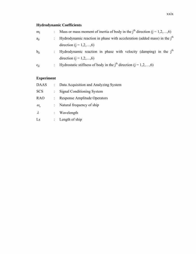
Hydrodynamic Coefficients
mj : Mass or mass moment of inertia of body in the jth direction (j = 1,2,…,6)
ajj : Hydrodynamic reaction in phase with acceleration (added mass) in the jth
direction (j = 1,2,…,6)
bjj : Hydrodynamic reaction in phase with velocity (damping) in the jth
direction (j = 1,2,…,6)
cjj : Hydrostatic stiffness of body in the jth direction (j = 1,2,…,6)
Experiment
DAAS : Data Acquisition and Analyzing System
SCS : Signal Conditioning System
RAO : Response Amplitude Operators
nω : Natural frequency of ship
λ : Wavelength
Ls : Length of ship
xxx
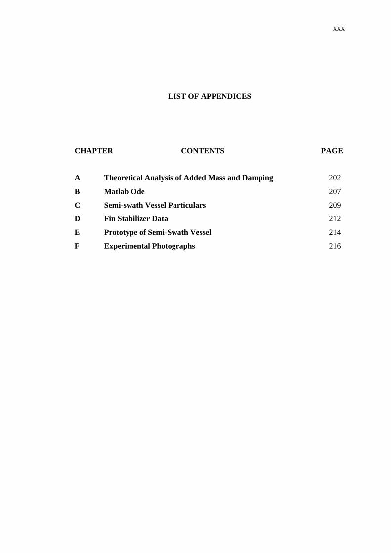
LIST OF APPENDICES
CHAPTER CONTENTS PAGE
A Theoretical Analysis of Added Mass and Damping 202
B Matlab Ode 207
C Semi-swath Vessel Particulars 209
D Fin Stabilizer Data 212
E Prototype of Semi-Swath Vessel 214
F Experimental Photographs 216
CHAPTER 1
INTRODUCTION
1.1 Background
The applications of twin-hull vessels particularly SWATH vessel and
conventional Catamaran have widely designed regarding for purpose of providing
better seakeeping quality than mono-hull vessels inherently.
Holloway and Davis (2003) and Kennell (1992) stated that inherent to the
advantages of SWATH vessels, as compared to the conventional Catamaran is its
smaller waterplane area that provided smaller wave excitation forces, lower
amplitude motion associated with its lower accelerations responses and better
seakeeping performances. Dubrovskiy and Lyakhoviyskiy (2001), Fang (1988) and
Kennell (1992) mentioned that the SWATH vessels have larger natural period as
twice as long the natural periods of roll, pitch, and heave of a mono-hull of
comparable size.
Based on Dubrovskiy and Lyakhoviyskiy (2001) and Ozawa (1987) have
presented the advantages of conventional Catamaran features compared to the
SWATH vessels have shallower draft and lower cost of construction. Their larger
waterplane areas as compared to the SWATH vessel has increased the stiffness as
result as improve vessel’s longitudinal stability.
2
Conversely, the particular drawbacks of SWATH vessel and conventional
Catamaran geometrically cannot be neglected. It is shown that the SWATH vessel
with its small waterplane area is tender in large pitch motion due to low stiffness
resulted as increase in speed. Djatmiko (2004), and Dubrovskiy and Lyakhoviyskiy
(2001), and Kennell (1992) stated that the low value of this parameter is linked to its
insufficient values of longitudinal metacentric height (GML). Consequently, this
may lead to pitch instabilities, which caused slamming, deck-wetness, excessive trim
or even bow diving and degrade the passenger comfortability.
Having considered some extensive reviews of several obtainable advantages
both SWATH and conventional Catamaran hull forms, an alternative hull form
design is proposed to overcome and minimize their drawbacks. The proposed design
concept represents a combination of conventional Catamaran and SWATH hull
features. In addition, this new modified hull form configuration conceptually was
emphasized on the variable draught operations i.e. shallow draught and deep draught.
Then, this vessel is called “Semi-SWATH vessel.”
Holloway (1998 and 2003) investigated that as the hybrid design hull form;
the Semi-SWATH configurations generally offered two ways that make the most of
Semi-SWATH vessel’s benefits. First, its primary premise is to maintain a good
seakeeping quality. Second, it is intended to prevent the bow diving phenomena at
high-speed. It means the maturity of Semi-SWATH vessel is going to provide an
improvement of conventional Catamaran and SWATH vessel drawbacks
considerably.
Furthermore, the placement both of fixed bow fins and controllable stern fins
on each lower hull of Semi-SWATH vessel will provide additional pitch restoring
moment to improve not only the longitudinal stability but also reduce the vertical
motion responses. Consequently, the serious inconveniences will degrade the vessel
performance during sailing especially at high-speed head sea waves can be
alleviated. Haywood, Duncan, Klaka, and Bennett (1995) stated that the seakeeping
of the Semi-SWATH vessel is going to be better evidently.
3
The simulation program of Semi-SWATH vessel incorporated with fixed fore
and controllable aft fins were developed to evaluate the seakeeping performance
during operation at both medium speed (15 knots) and high-speed (20 knots). The
mathematical model comprising of heave and pitch motions, which incorporated with
the fins stabilizers on the simulation was presented in a simple block diagram using
Matlab-SIMULINK. In this simulation, a conventional PID controller was
developed and applied on the controllable aft fins. Segundo, et al (2000) developed
simulation program using PID controller to alleviate vertical accelerations due to
waves. The results of simulation had been validated by experiments in the towing
tank confirm that by means of flaps and a T-foil, moved under control, vertical
accelerations can be smoothed, with a significant improvement of passengers
comfort. In addition, Caldeira, et al (1984), Ware, et al (1980a), (1980b), 1981, and
1987, and Chinn, et al (1994) applied conventional optimal PID controller design to
improve the vertical motion response of marine vehicles.
In this PID controller method, some parameter of tuning controller will
involve some chosen controller gain parameters of PID (Kp, Ki, and Kd are the
proportional, integral, and derivative gains, respectively). Those parameters are
obtained using method of Aström and Hagglund. Then, they will be considered to
satisfy certain control specifications by minimizing the error after achieving steady
state. This controller mode is applied by controlling the aft fin’s angle of attack
properly, the sailing style of Semi-SWATH vessel must be adjusted to be in even
keel condition. The theoretical prediction results will be validated with the model
experiments carried out in the Towing Tank of Marine Technology Laboratory,
Universiti Teknologi Malaysia.
1.2 Research Objective
1. To evaluate the seakeeping performance of Semi-SWATH vessel before
and after installation both of fixed fore and controllable aft fins in regular
head sea using time domain simulation and validated by model test in
Towing Tank.
4
2. To apply a ride control system on the controllable aft fins, the
conventional PID controller will be used to achieve a better quality the
Semi-SWATH seakeeping performance.
1.3 Scopes of Research
1. The mathematical dynamics equations model covers Semi-SWATH
vessels with fins in two degrees of freedoms i.e. heave and pitch motions
operating in regular head sea.
2. The numerical method simulation is based on Time-Domain using
Matlab-SIMULINK.
3. In the simulation, the regular waves generated using MATLAB for any
wavelength of interest as well as experiment done (range of regular wave
lengths: 0.5 ≤ λ/L ≤ 2.5 and steepness of the incident wave: H/λ = 1/25)
4. The hydrodynamic coefficients of Semi-SWATH vessel motions will be
obtained using numerical program, which was developed by Adi Maimun
and Voon Buang Ain (2001).
5. The proper fin stabilizers were selected using NACA-0015 section due to
high lift curve slope and low drag.
6. Coefficient of Lift (CL) previously will be obtained using CFD software
(Shipflow 2.8).
7. A conventional PID controller will be applied on the Semi-SWATH
vessel to improve the stability and performance of plant system with
adequate reliability.
8. A parameter tuning of PID controller is obtained using method of Aström
and Hagglund i.e. Kp, Ki, and Kd. Then, they will be applied to satisfy
certain control specifications by minimizing the error after achieving
steady state.
9. The simulation program result will be validated of by the Semi-SWATH
model test carried out in Towing Tank of Marine Technology Laboratory,
Universiti Teknologi Malaysia.
5
1.4 Research Outline
An achievement of the excellent seakeeping qualities for ship design requires
extensive consideration as guidelines to reflect the safety, effectiveness, and comfort
of vessel in waves. The present research follows a systematic procedure to modify
concept design of twin-hull vessel by minimizing their drawbacks. This study starts
from the review of SWATH and conventional Catamaran hull forms. The final
design of the new modified hull form will deal to enhance the vessel’s stiffness
associated with improving seakeeping qualities at high-speed in head seas waves
condition. Then this vessel is called Semi-SWATH vessel.
The flexibility of the Semi-SWATH vessel can be operated in two variable
draughts i.e. shallow draught and deep draught with still maintain seakeeping quality.
In these variations of operational draughts, the Semi-SWATH vessel will be operated
in two speed services i.e. medium speed (15 knots) and high-speed (20 knots).
Furthermore, the effects of vertical motions on the Semi-SWATH vessel (heave and
pitch motions) when encountering head sea at those service speed will be
investigated considerably.
For this reason, an advanced prediction analysis both numerically and
experimentally to achieve a desired goal will be done. In stage of the Time-Domain
Simulation approach theoretically will be used to predict and analyze the seakeeping
performance in head sea waves, which was developed using Matlab-SIMULINK.
Then, the mathematical model comprising of heave and pitch coupled motions before
and after attached fixed bow and active stern fin stabilizers are investigated. Then,
the conventional PID controller is applied on the active stern fin stabilizer by tuning
its angle of attack to enhance the improvement of ride quality ideally to be even keel
riding condition. Then, the real-time simulation results will be validated by
experimental model test carried out in Towing Tank at Department of Marine
Technology, Universiti Teknologi Malaysia.
Finally, the seakeeping evaluation of Semi-SWATH vessel is identified based
on the motion response, which presented by Response Amplitude Operators (RAOs).
6
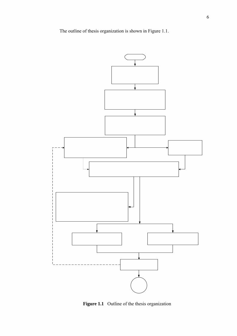
The outline of thesis organization is shown in Figure 1.1.
Figure 1.1 Outline of the thesis organization
CHAPTER 2
LITERATURE REVIEW
2.1. General
The aim of this chapter is to give an overview and the assessment method to
evaluate seakeeping performance of the Semi-SWATH vessel. The extensive
reviews of the pertinent literature have been done to obtain a useful information and
methodology for this work. This thesis is organized in six sections, as follows; the
first section is to provide a better understanding of the basic design of Semi-
SWATH vessel modified between SWATH vessel and Catamaran. The second
section treats on the critical review of the twin-hull vessel due to effect of vertical
motion i. e. pitch and heave motion. These motions primarily have a significant
effect to dynamic stability criteria especially at high forward speed. The additional
feature of cross-structure submergence with a bow-diving of Semi-SWATH vessel
add to the severity which degrade comfortability and structural damage with greater
safety risks. The third section is to evaluate the effect of pitch stabilization on the
vessel motions during operation. The fourth section utilizes the development of a
rationale simulation control systems of fin stabilizers. The conventional PID
controller will be established. The fifth section is the critical review of the existing
seakeeping criteria of Semi-SWATH vessel as a type of twin-hull vessel.
8
2.2. Historical Design of Semi-SWATH vessel
Early, the development of twin-hull high-speed vessels naturally focused on
developed a reputation for poor seakeeping performance when encountering head sea
at high forward speed. Beaumont and Robinson (1991), Brown, Clarke, Dow, Jones
and Smith (1991) and Roberts, and Watson and Davis (1997) stated that this bad
reputation was shown by their tendency for larger pitch motions or even bow diving
and more severe dynamic structural loads than for mono-hull vessels. Consequently,
they will threat the vessel comfortability and safety.
Inherently, several solutions have been attempted to improve their
performances particularly to minimize their drawbacks and risks. One of the
solutions have been proposed is create or modify a new hull form design. In this
thesis, the author had endeavored to develop an alternative design hull forms or
modified design of twin-hull vessel hull forms to meet those requirements. This new
design hull form will not only maintain the quality of good seakeeping performance
in seaway but also directly is able to minimize the large pitch motion by increasing
the vessel’s stiffness longitudinally. Thus, some extensive reviews of twin-hull
vessels especially for Catamaran and SWATH vessel have been studied considerably.
Where, the coupled mother vessel between a SWATH vessel and Catamaran vessel
result a new genetic vessel design of a Semi-SWATH vessel.
2.2.1 Catamaran
Dubrovskiy and Lyakhoviyskiy (2001) explained the local term “katto
maram”, meaning “coupled tress”, become the commonly accepted word Catamaran.
The principle of the Catamaran vessel geometrically is the connecting structure
between the two hulls was used for navigation and became known as "the bridge" or
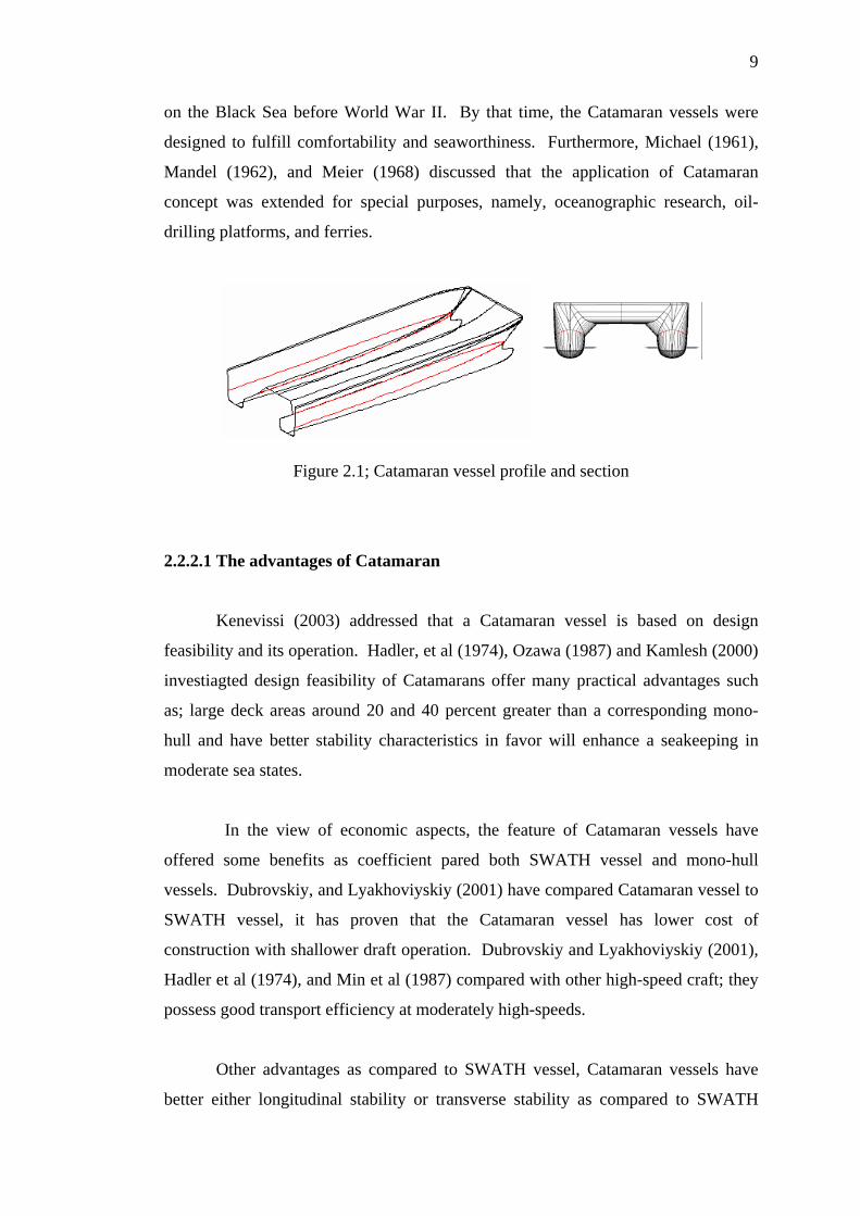
cross deck. The modern feature of Catamaran vessel can be seen at figure 2.1.
In the recent decades, the research and development of Catamaran vessels
had widely spread in world; Japan, USA, UK, Australia, Norway, Russia etc.
Gartwig (1974) stated that the first Russian high-speed Catamaran Express was built
9
on the Black Sea before World War II. By that time, the Catamaran vessels were
designed to fulfill comfortability and seaworthiness. Furthermore, Michael (1961),
Mandel (1962), and Meier (1968) discussed that the application of Catamaran
concept was extended for special purposes, namely, oceanographic research, oil-
drilling platforms, and ferries.
Figure 2.1; Catamaran vessel profile and section
2.2.2.1 The advantages of Catamaran
Kenevissi (2003) addressed that a Catamaran vessel is based on design
feasibility and its operation. Hadler, et al (1974), Ozawa (1987) and Kamlesh (2000)
investiagted design feasibility of Catamarans offer many practical advantages such
as; large deck areas around 20 and 40 percent greater than a corresponding mono-
hull and have better stability characteristics in favor will enhance a seakeeping in
moderate sea states.
In the view of economic aspects, the feature of Catamaran vessels have
offered some benefits as coefficient pared both SWATH vessel and mono-hull
vessels. Dubrovskiy, and Lyakhoviyskiy (2001) have compared Catamaran vessel to
SWATH vessel, it has proven that the Catamaran vessel has lower cost of
construction with shallower draft operation. Dubrovskiy and Lyakhoviyskiy (2001),
Hadler et al (1974), and Min et al (1987) compared with other high-speed craft; they
possess good transport efficiency at moderately high-speeds.
Other advantages as compared to SWATH vessel, Catamaran vessels have
better either longitudinal stability or transverse stability as compared to SWATH
10
vessels and mono-hull vessels. Dubrovskiy and Lyakhoviyskiy (2001) state that the
better longitudinal stability (GML) is offered by larger waterplane area as
consequence as increased the vessel stiffness. In addition, due larger waterplane
areas at the bow results more buoyancy forces, which can reduce the pitch motion as
compared to the SWATH vessel. Thus, the tendency of Catamaran to the bow diving
can be minimized. Dubrovskiy and Lyakhoviyskiy (2001) has investigated that the
transverse metacentric height of Catamaran is 8-10 times greater than comparable
mono-hull.
2.2.1.2 The drawback of Catamaran
Inherent to feature of Catamaran due to larger beam has negative effect to the
performance in seaway. Comparing the vertical deck edge acceleration, wave
excitation finds considerably larger amplitudes for the Catamaran than the mono-hull
vessel. This is probably caused by the fact that the two fore-bodies of the Catamaran
in bow sea encounter the wave crest with a certain difference in phase, which is
unfavorable. Khristoffer (2002) investigated that Catamarans has revealed to the
cross-structure slamming problems in seaway. Consequently, Hadler, et al (1974)
had shown that Catamaran has a limited operation because of the cross-deck
structure will have local indentations or even rupture.
Other drawback of the Catamaran geometrically in waves is higher wave
resistance components compared to mono-hull. Molland et al. (1994) and (1996)
gave evidence and found approximately 10% greater form factor than mono-hull due
to viscous interaction effect. This phenomenon was caused by owing to high wetted
surface area and hence skin fiction drag. Accordingly, Catamaran will require more
high power for ocean going and its construction cost is slightly higher compared to
mono-hull vessel.
11
2.2.3 SWATH vessel
The initials S.W.A.T.H. stand for Small Waterplane Area of Twin Hull. The
SWATH vessel is a relatively recent development in ship design. Kennell (1992),
the superior seakeeping quality is usually the primary motivation for considering
SWATH vessel. Although patents employing this concept show up by Nelson
(1905), Blair (1929), Faust (1932), Creed (1946), Leopold’s (1969), and Lang (1971).
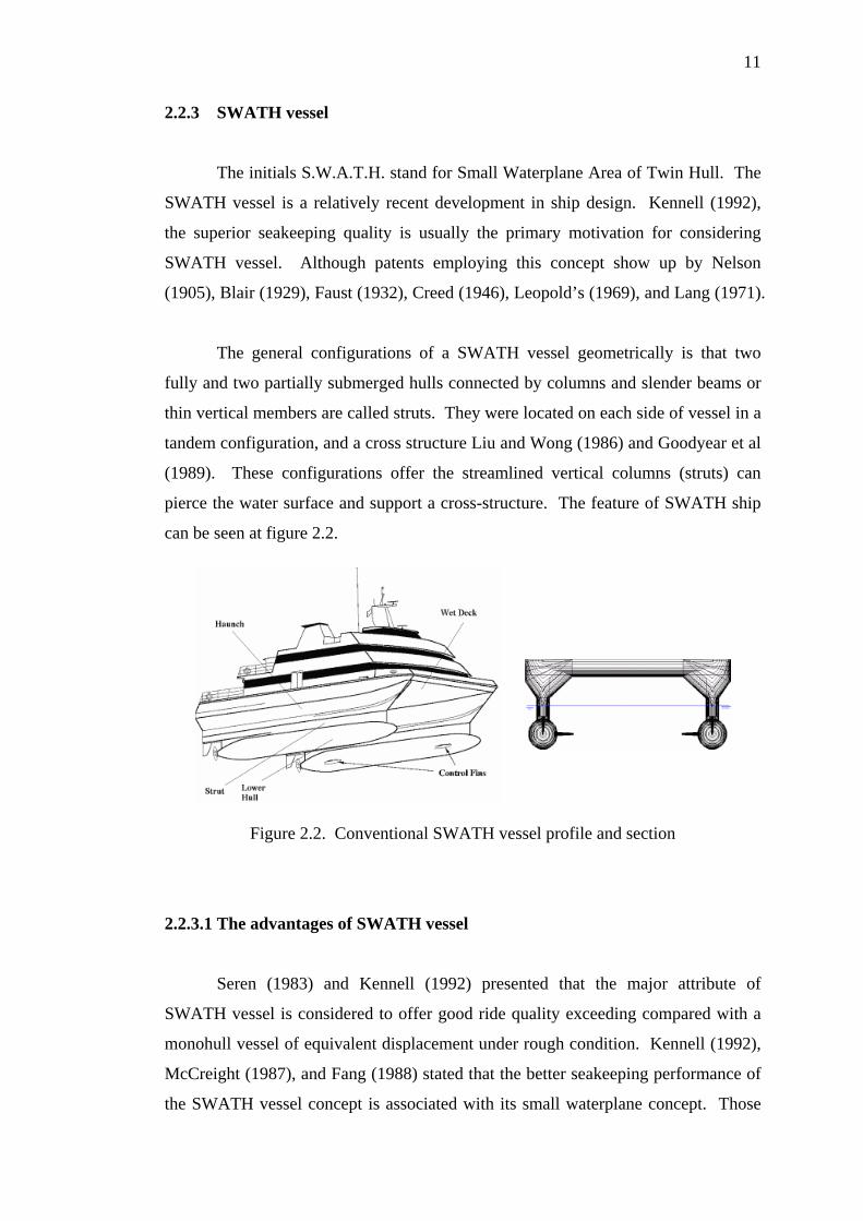
The general configurations of a SWATH vessel geometrically is that two
fully and two partially submerged hulls connected by columns and slender beams or
thin vertical members are called struts. They were located on each side of vessel in a
tandem configuration, and a cross structure Liu and Wong (1986) and Goodyear et al
(1989). These configurations offer the streamlined vertical columns (struts) can
pierce the water surface and support a cross-structure. The feature of SWATH ship
can be seen at figure 2.2.
Figure 2.2. Conventional SWATH vessel profile and section
2.2.3.1 The advantages of SWATH vessel
Seren (1983) and Kennell (1992) presented that the major attribute of
SWATH vessel is considered to offer good ride quality exceeding compared with a
monohull vessel of equivalent displacement under rough condition. Kennell (1992),
McCreight (1987), and Fang (1988) stated that the better seakeeping performance of
the SWATH vessel concept is associated with its small waterplane concept. Those
12
advantages were naturally provided by a stable platform in seaway and their features
indicate significantly minimizing a drag as well as keeping the resistance down, low
wave excitation forces, greatly reduced deck motions exhibited while at rest or
underway, lower accelerations for given amplitude of motion, eliminate the
seasickness, and give the vessel mobility comparable to mono-hulls.
Inherent to their operational draughts, the SWATH vessel has deeper draught
than Catamaran vessel with comparable displacement. Seren (1983) presented an
advantage to this feature considered be able to offer medium speeds, a wide stable
platform with good stability, and good seakeeping ability exceeding that of much
larger conventional mono-hull vessels under rough sea conditions.
Ozawa (1987) summarized advantages of the SWATH ships inherently
compared with the equivalent monohull vessel can be taken as follow:
(i) less motions and acceleration by waves, longer resonant frequency
characteristic of larger monohull vessels; especially as the rolling resonant
frequency is very long, motions and acceleration by waves are less than for
conventional hulls.
(ii) less speed loss in rough seas than conventional vessels because of minimal
pitching motions.
(iii) directional stability and maneuverability at both low and high speeds are good,
owing to the widely separated struts and the effective differential thrust system.
(iv) good intact and damage stability due to large reserve buoyancy of the strut’s
flare and the deck and also moderate ballasting system.
The above cited activities and advantages of the SWATH vessel design concept
support a belief in its unique capabilities and practicability over a broad range of
missions.
2.2.3.2 The drawback of SWATH vessel
The seakeeping of SWATH vessels are gained at some sacrifice. Holloway
(2003) explained that the increased motion amplitudes of SWATH vessel due to an
13
increased wave force associated with the longer wavelengths is possible to occur
resonant motions. Furthermore, the lower natural frequency means that resonance
occurs in longer waves, also contributing to longer motions.
Djatmiko (2004), Dubrovskiy, and Lyakhoviyskiy (2001), McCreight (1987)
and Clark, et al (1990) explained in the view of safety aspect, the significant
drawback accompanied with low waterplane area. This feature was caused the
SWATH vessel has more sensitivity of draught to changes in weight during design
and operation. It means, the low waterplane area brings about reduction in the
moment to change trim, which also means low hydrostatic restoring moment, hence
makes the vessel vulnerable towards pitch instabilities due to dropped or low
restoring pitch moment resulted as increase in speed.
Another problem of the SWATH hull form in view of the commercial
viability has caused the higher cost of construction. McGregor (1992) and Ozawa
(1987) presented thatt, the SWATH vessel is still prohibitive due to require very high
power to cruise at moderately high-speeds. This problem was caused by the greater
wetted surface that disproportionately deeper draught as compared to mono-hull or
Catamaran, Kennell (1992).
Ozawa (1987), summarized disadvantages of the SWATH ships inherently
compared with the equivalent monohull vessel can be taken as follow:
1) an increase in propulsion power due to its greater wetted surface area which
causes an increase of frictional drag.
2) sensitivity to trim and heel changes by weight ship on deck due to its small tones
per centimeter properties, and comparatively small metacentric height it requires
more severe KG allowances in the design stage than conventional vessels, ballast
compensation systems or necessary for a SWATH ship.
3) a greater draught causing docking and restricted draught problems, especially in a
large SWATH ship.
4) in the case of vessel built of steel, a smaller ratio of payload to structural weight
compared with the equivalent conventional displacement type monohull vessels.
5) relatively larger turning diameter in relation to length in a high speed SWATH
ship.
14
2.3 The Concept of the Semi-SWATH vessel
Based on the reviewing both SWATH vessel and Catamaran vessels are
driving the search for new design concept, which had better satisfy design
requirements. Those were shown by, SWATH and conventional Catamaran vessels,
which provide several obtainable advantages.
Shack (1995) began from the review of conceptual design of fast passenger
vessels that involves several unsolved problems regarding resistance, propulsion,
seakeeping and passenger comfort. The objective of this study has been to establish
a broad view of the concepts that could possibly be used to produce a new generation
of high-speed passenger of the future. The study includes mono-hulls, Catamarans,
SES (Surface Effect Ship), SWATH vessel (Small Waterplane Area Twin Hull).
Then, he proposed a hybrids hull form with very promising results and would
therefore serve as a good platform. Then this vessel is called the Semi-SWATH
vessel.
Atlar (1997) had been studied comprising with Catamaran and SWATH
vessel designs. He recommended a new concept of vessel design is to minimize the
vessel responds to any disturbances, producing a harsh and so-called “stiff” ride
especially at high-speed as compared to SWATH vessel. As may be known, the
vessel’s stiffness has significant effect of creating high absolute vertical accelerations,
a well-known cause of motion sickness. Joseph, et al (1984) and Atlar (1997), they
proposed a mutation of generation hull form that conceptually is still taking the small
waterplane area of twin-hull (SWATH) on hull form designs. Then, this vessel is
called Semi-SWATH vessel.
Holloway (2003) presented that the semi-SWATH idea is an obvious
opportunity to exploit the positive aspects of both SWATH and conventional
Catamaran hull forms. Gaul, et al (1984, 1987, 1994, and 1988), Lang, et al (1979)
and Holloway (2003) investigated that conceptually this design also was emphasized
on the variable draught operations to minimize the single draught of SWATH vessel
and to trade off performance and seakeeping. The primary objective of Semi-
15
SWATH vessel is to give the best possible ride in a seaway, especially when the
vessel is adrift, holding station, or underway at low speeds.
Holloway (2003) developed the fundamental concept design relating to semi-
SWATH geometrically is emphasized on the waterline beam reduction for the whole
length of the boat or only for part of the length (for example only for the forward
half). There is considerable scope for variations, and as yet there is no “normal”
semi-SWATH design. In the view of his concept design, the distinction between a
SWATH and a conventional hull is that the waterplane area in the former should be
smaller than the maximum submerged plan area that is the waterline beam for at least
some sections is smaller than maximum beam at the same sections. On other hand,
Kristoffer Grande (2002) had considered the same background design to find a better
seakeeping performance of twin-hull vessels in seaway. He has proposed a design of
the Semi-SWATH vessel hull conceptually by reducing the waterline line width in
the bow, and produces a very fine entry.
2.3.1 Advantages of Semi-SWATH vessel
Holloway, (1998) and (2003) investigated that generally the design concept
of Semi-SWATH vessel configuration offered two ways that make the most of Semi-
SWATH vessel’s benefits. First, its primary premise is to maintain a good
seakeeping quality. Second, it is intended to prevent the deck-diving phenomena at
high-speed. It means the maturity of Semi-SWATH vessel is going to provide an
improvement of conventional Catamaran and SWATH vessel drawbacks
considerably.
In the view of seakeeping quality, Gaul (1988), the Semi-SWATH vessel or
Semi-Submerged ship has promised to provide a better operability for overboarding
in high sea states. Gaul (1988), Coburn (1995) and Holloway (2003) presented a
better seakeeping quality was achieved due to variable range of her draught mode
operations, which is able to trade off the performance and seakeeping quality
accordingly. These were shown, in the view of SWATH mode (deep draught
condition with ballasting system) is evident greatly to the reduced waterplane area
16
and deck motions exhibited while at rest or underway. This draught mode gives the
steadiest platform for slow and medium speed operations incident rough sea
conditions in deep water. Holloway (2003) gave a reason that the Semi-SWATH
vessel provides for lower the natural frequencies of heave and pitch response as well
as less wave-exciting forces. In addition, Davis and Holloway (2003) stated that the
SWATH mode will give benefit in order to reduce the magnitude of motions
particularly in the forward parts of the vessel. McGregor (1992), Lang (1988) stated
that the greatly reduced pitch motions will improve seakeeping quality while at rest
or underway. Gaul (1988) studied even in the deeper draught, the seakeeping quality
of Semi-SWATH vessel can be superior to an equivalent SWATH vessel.
In the view of preventing a deck-diving phenomenon at high-speed was
offered in her operational mode (conventional Catamaran mode). Holloway and
Davis (2003) explored in this mode, the Semi-SWATH vessel will exist to be
operated in shallow draught conditions such as in estuary area and sheltered water
with unique deballasting system appropriately. The condition of shallow draught is
set up for a transit draught where it is fully loaded with the ballast tanks empty. As
results, this feature is especially useful during transit to permit higher speeds. The
configuration by enlarging waterplane area of vessel has substantially increased the
hydrostatic stiffness relative to the ship mass as consequence as satisfy the
seakeeping design objectives especially at high-speed that SWATH vessel cannot do.
As a result, the vessel’s tendency to an excessive trim or even bow diving when
encountering head seas at high-speed can be reduced. Gaul (1979) presented other
advantages of Semi-SWATH vessel is due to capitalized on wide footprint, generous
deck space, and trim flexibility to give low motion profile.
2.3.2 Motion Response of Semi-SWATH vessel
Holloway (2003), Lang (1979) and Gaul (1988) presented that the dominant
advantage that the Semi-SWATH vessel or Semi-Submerged vessel offers is drastic
reduction in ship motion. Gaul (1988), the improved seakeeping is provided in both
the transit mode and, more importantly, during on-station research operations. This
motion response reduction allows the Semi-SWATH vessel to operate in much
17
higher seas than can be tolerated with an equivalent mono-hull. The radical
decreases in waterplane area above the lower hull reduce buoyant forces caused by
wave action and ameliorate motion response. It should be noted that this is a key
difference between a Semi-SWATH vessel and a conventional Catamaran vessel.
Holloway (2003) studied on two model tests that the Semi-SWATH vessel or
Semi-Submerged ships, even at transit draught, will have lower motion response that
a comparable conventional hull. Gaul (1988) explained that in beam seas, the roll of
mono-hull can be more than five times higher than that of Semi-SWATH vessel. In
pitch, the mono-hull response typically is two to three time higher. This feature
alone prompts the consideration of Semi-SWATH vessel in place of mono-hulls for
passenger vessels.
Gaul (1988) stated that the response of the vessel to a seaway is highly
dependent on wave periods or, more precisely, on encounter frequency, which is a
function of wave frequency, vessel speed, and relative heading. When underway in
head seas, the apparent encounter frequency is longer than wave frequency, so vessel
motions are very small. On the contrary, when the apparent frequency is shorter than
wave frequency, the Semi-SWATH vessel motions are very long. As results will
cause exceed deck motion as threshold for seasickness discomfort.
Schack (1995) studied on the demihull series of hull forms. He developed
ranging from the pronounced Semi-SWATH hull form to a conventional high-speed
catamaran with a typical U-shape. Due to there being very little interference and
interaction between the demihulls both regarding resistance and seakeeping, it was
decided that the calculation and model test should be carried out with the demihull
only, this was furthermore validated via the model test program. On the basis of the
small systematic study conducted via numerical calculations and model tests, it can
be concluded that the Semi-SWATH hull form in the most probable sea states is
superior to the conventional catamaran hull forms.
Holloway (1998) has summarized the response related to model test of Semi-
SWATH vessel in Towing-Tank, as follow;
18
• as speed is increased motions also increase, primarily due to the increased forcing
resulting from encountering resonance in longer waves, but only to the point
where the resonant frequency is encountered in wavelengths significantly longer
than the boat length, in which case the motions are asymptotic to their maximum
value. This means that at high-speeds poor seakeeping is inevitable for all hull
types (excluding the effect of appendages).
• for the same reason increasing SWATHness (waterplane area reduction) also
increases motions. However, the lower natural frequency of SWATHs at the
same time reduces accelerations, and this to some extent cancels the effects of the
increased motions. The increased motion effect dominates at low speeds where
the rate of change of forcing with frequency at the natural frequency is high, but
at high speeds where it is asymptotic (and therefore changes only slowly with
frequency) the lower acceleration effect dominates.
2.4. Prediction of Ship Motion
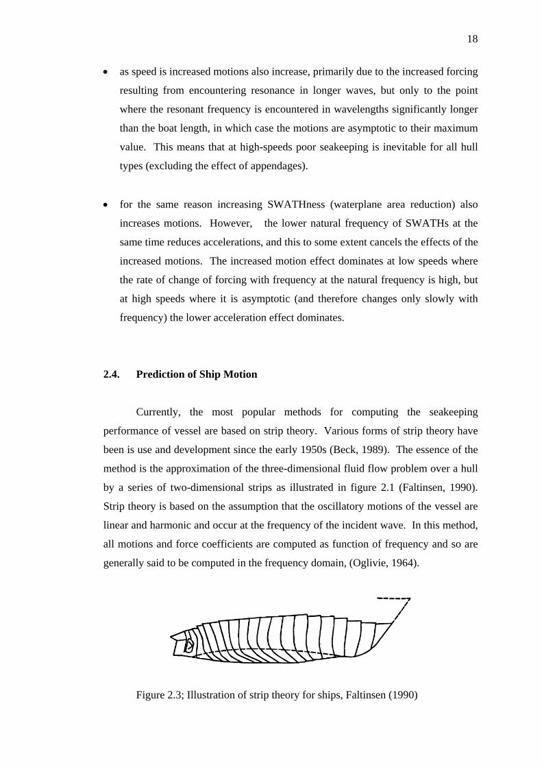
Currently, the most popular methods for computing the seakeeping
performance of vessel are based on strip theory. Various forms of strip theory have
been is use and development since the early 1950s (Beck, 1989). The essence of the
method is the approximation of the three-dimensional fluid flow problem over a hull
by a series of two-dimensional strips as illustrated in figure 2.1 (Faltinsen, 1990).
Strip theory is based on the assumption that the oscillatory motions of the vessel are
linear and harmonic and occur at the frequency of the incident wave. In this method,
all motions and force coefficients are computed as function of frequency and so are
generally said to be computed in the frequency domain, (Oglivie, 1964).
Figure 2.3; Illustration of strip theory for ships, Faltinsen (1990)
19
Many of the early methods were limited to zero speed, head seas or motion in
the vertical plane only. During 1969 and 1970, several papers were published by
different groups working independently which introduced more general forms of the
theory including Söding (1969), Tasai and Takaki (1969) and Borodai and
Nesvetayev (1969). The method described by Salvesen et al. (1970) has been the
most widely accepted (Beck, 1989). All these new strip theories have identical
forward-speed terms satisfying the Timman and Newman symmetry relationships,
and, interestingly enough, the equations of motion for heave and pitch in head waves
derived in the present work have the same speed terms. This method also includes
prediction of sway, roll, and yaw motions as well as wave induced loads a ship at
constant speed at an arbitrary heading in regular waves.
There are three main stages to computing the ship’s response using strip
theory. First, the ship is divided into a number of transverse sections or strips,
typically numbering twenty to forty. Second, the two-dimensional hydrodynamic
coefficients (added mass, damping, wave-excitation and restoring force) are
computed for each section. Third, these values are then integrated along the length
of the vessel to obtain the global coefficients for the couple vessel motions. Finally,
the equations of motion are solved algebraically.
Two methods are commonly used to calculate the hydrodynamic forces on
the strips: are conformal mapping and Close-Fit methods. In the first method, the
section coefficients are calculated by relating the actual section shape, via a
conformal mapping, to that of a union semi-circle for which the solution is known.
Various methods have been proposed to perform this mapping such as those of Lewis
(1929) and Ursell (1949). The most commonly used of these is based on the Lewis
forms which use two parameters based on the sectional beam-to-draft ratio and the
sectional area coefficient to define the mapping.
Close-fit methods are those, which attempt to solve the potential flow
problem directly on the actual sectional geometry using boundary integral techniques.
The method Frank (1967) is perhaps the most commonly used of these methods. The
Frank Close-fit method represents the section shape as a series of straight-line
segments. A series of fluid sources of constant but unknown strength are distributed
20
along each segment. Applying the boundary conditions permit solution of the source
strengths and hence the velocity potential on each segment. The pressure associated
with the velocity potential is then integrated over the surface of the section to yield
the added mass and damping coefficients.
While the formulation of strip theory assumes a long, slender (Faltinsen,
1990), its use for alternate hull forms was anticipated by Salvesen et. al. (1970) over
thirty years ago. The method has subsequently been applied to more complex hull
forms including, Catamaran, SWATH vessel and others types of multi-hull vessels.
The method has been proven to provide reliable estimates of motions and hull loads
for a surprisingly wide range of hull forms and sea conditions as evidenced by the
wide range of engineering software products in use today. A theoretical method for
predicting the ship motions in waves was applied to the Semi-SWATH vessel for
similar to that applied to SWATH vessel (Lee, 1976). He applied a conventional
strip theory of Salvesen, Tuck and Fatilsen to twin-hull ship in order to develop
potential flow coefficient. Where, he has developed the SWATH vessel motion
prediction in waves using strip theory with involving with three main extra
considerations included in the hydrodynamic coefficients.
1. the hydrodynamic interactions between two-hull.
2. effect of viscous damping. It is of the same order of magnitude of the wave
making damping. Consequently neglecting it results in twin-hull system being
under damped.
3. effect of stabilizing fins. A Semi-SWATH vessel can become unstable in pitch
above a certain speed. The longitudinal unsymmetrical pressure distribution on
the two lower hull produce a destabilizing moment causing the vessel to “bow
down.” The moment is called the “munk-moment” and is proportional to the
square of the speed. This associates needs for compensating stabilizing fins. The
fins also help damping through hydrodynamic lift. Therefore, a Semi-SWATH
vessel is not viable without fins and their effects must be included in any
calculations of motion.
21
2.5 Motion Characteristics of High-Speed Vessels
The Semi-SWATH vessel is known to offer a high quality in low and
moderate sea states compared to conventional Catamaran. However, high-speed
Semi-SWATH vessel in heavy sea states there are problems with discomfort owing
to high frequency vertical accelerations especially due to large heave and pitch
motions. Furthermore, the lower natural frequency means that resonance occurs in
longer waves, also contributing to larger motions, Segundo, et. al (1999 and 2000).
Therefore, a reduction in heaving and pitching will in general improve comfort for
passengers.
In addition, designers and builders are starting to see the benefits of better
seakeeping not only in terms of passenger comfort but also in terms of dynamic
structural safety problems. Christoffer (2002) had shown that slamming and deck
wetness events are likely to be both more severe and more frequent than for mono-
hull vessels at high forward speeds. Consequently it is not only degrade the vessel
performances but also damage the structure with greater risk. This phenomenon was
occurred on a high-speed vessel, which receives a not inconsiderable amount of lift
forward from the spray rails. Tank tests have shown that, once a certain speed is
exceeded, these may cease to deflect the bow wave or spray and become engulfed.
When this happens, the bow may drop, to the accompaniment of large sheets of
green water thrown into the air in the region of the fore body.
Therefore, the evaluations of motion characteristic of high-speed twin-hull
vessel particularly due to large vertical motion (heave and pitch motions) a will be
taken respectively in a present considerable research that has already undertaken in
the area.
2.6 The Effect of Heave and Pitch Motion Responses
Goodrich (1968), during operation, the heave, and pitch motions would
routinely influence to the magnitude of vessel. The effects were concerned to the
parametric their large excitation motions as considered as critical situation suffered
22
by the vessel. As results, they will generate wave impacts on the bottom of the cross
structure of a Semi-SWATH vessel, as well as the usual problems of deck wetness on
the forecastle or of slamming on the forefoot. The motion of ships in the sea was
violent, pitch ± 8 degrees being commonplace. Sariöz and Narli (2005), for a
passenger vessels, vertical motions (heave and pitch motions) are of main concern
due to effect of accelerations on the comfort and well-being of the passengers.
Ozawa (1987), hence, their large vertical motions affected to high accelerations,
which deal to affect some negative aspects on the vessel during operation, such as
slamming.
Djatmiko (2004) stated that as the twin-hull vessels, the small waterplane
area at the bow of SWATH vessel at high-speed operation will cause large pitch
motions as consequence as more sensitive to trim and heel changes by weight ship on
deck due to its small tones per centimeter properties, and comparatively small
metacentric height. Further, the low waterplane area due to heave and pitch motions
bring about reduction in the moment to change trim, which also means low
hydrostatic restoring moment, hence makes the vessel vulnerable towards pitch
instabilities.
Kenevissi (2003) explained that the large tendencies heave and pitch motion
of the SWATH vessel in high forward speed produces a harsh stiff ride or low
restoring moment. Where, this stiffness has the effect of creating absolute vertical
motion acceleration. The low value of restoring moment is linked to its values of
longitudinal metacentric height (GML). In addition, the insufficient of GML may
experience a static trim and at the same endure a much sinkage compared to its
draught. Djatmiko (2004) was shown, on top of that, sinkage and static trim
naturally yields an increase in total resistance due to involuntarily additional wetted
surface area. Katayama, (2002b), Djatmiko (2004), Dubrovskiy and Lyakhoviyskiy
(2001) presented that those phenomena occurred when hydrodynamic forces are
dominant compared with hydrostatic forces like buoyant forces.
Further effect of pitch and heave motions to the Semi-SWATH vessel
particularly at her operational modes has different characteristics subjected to the
vessel’s motion responses. In the conventional Catamaran mode, its larger
23
waterplane area has effect to reduce the dynamic instability of vessel’s motions
above a certain critical speed. Oppositely, on the SWATH mode, its small
waterplane area will affect on the minimizing of wave-exciting forces. As a result,
the Semi-SWATH vessel has relatively less resistance and longer natural periods of
heave or pitch motion compared to Catamaran. McCreight (1987), these longer
natural periods of motion enable the vessel to avoid resonant motions resulting from
wave-excitation forces in normally encountered seas.
Inherent to the geometry of the Semi-SWATH hull form is maintaining the
waterline line width as SWATH hull form characteristic in the bow produces pitch
motion. Excessive pitching on the relative vertical motion in the bow has strongly
influenced by sea conditions, in terms of ship motions and relevant sea loads, causing
uncomfortable conditions for passengers and hazardous situation for structural
integrity. Fan and Xia (2002), Esteban (2000), ISO (1995) and (1997), Dubrovskiy
and Lyakhoviyskiy (2001), and Davis and Holloway (2003) were shown in the worst
condition as a softer bow end responses make the vessel more prone to bow diving in
head seas and to a loss of longitudinal stability.
2.7 Pitch Motion Stabilizations
A high-speed vessel is riding in seaway with longer wavelength (one to two
times as long as the length of vessels) will take some unacceptable motion responses.
This results in severe pitching motion of high-speed vessels.
Abkowitz (1959), Bhattacarya (1978) and Conolly and Goodrich (1968)
discussed that the severe pitching motions of ships, particularly in head seas, are
responsible for loss of speed for a given power, for slamming with its associated risk
to the structure, motion sickness and possible injury to humans and damage to
equipment from the high accelerations that can be produced. Dubrovskiy and
Lyakhoviyskiy (2001) and Kennell (1992) discussed as well as twin-hull vessels,
inherently the SWATH vessels have limitation factors due to unacceptable pitch
motions particularly in high-speed operations. The unacceptable pitch motions have
often characterized by vertical struts of Semi-SWATH vessel designs (SWATHness
24
mode) during underway due to inherent small pitch damping. This pitch instability
was occurred due to its insufficient values of longitudinal metacentric height (GML)
resulted as increase in speed.
In addition, Fairlie-Clark (1990), Hadler, et al. (1974), Pinto, et al. (2001)
investigated a hydrodynamic force on the lower hull of SWATH vessel configuration
is susceptible to trim changes. Liu and Wong (1986), Papanikolaou (1991) presented
a result that the destabilizing bow down pitch moment (munk-moment) phenomenon
is generated as consequence as a pitch-instability can therefore occur at higher
speeds, while the normal static restoring force due to the waterplane is dependent
only on the pitch angle and ship speed. Holloway and Davis (2003) had studied that
in this situation the seakeeping quality of ship is poor because of resonance occurring
in combination with significant wave excitations.
By comparison, Semi-SWATH vessels have lower wavemaking damping in
all modes of motions as compared to mono-hull vessels. Since, the motions of Semi-
SWATH vessel produce little wave excitation action. For this reason, the motions of
Semi-SWATH hulls are lightly damped and can produce large responses if excited at
their natural periods. Kennell (1992) and Sariöz and Narli (2005) stated that
negative aspects of these large motions can be avoided by selecting natural periods
different from the most probable wave encounter periods or providing additional
damping forces to limit resonant responses. Therefore, the pitch instability must be
corrected in order to allow operation of the vessel above a certain critical speed.
In general, many efforts have been attempted to overcome such a problem,
and the most potential method attained is by introducing the anti-pitching fins.
Bhattacarya (1978) and Kennell (1992) stated that the one device that very useful and
currently used to minimize unacceptable pitching motions or pitch instability
resulting from high forward speed is the anti-pitching fin. Since, this device can
increase the hydrostatic stiffness of the vessel, which have much less effect at higher
and lower frequencies. Holloway (1998) explained that this of course refers to the
bare hull, and damping can be significantly increased with the use of fixed fins, and
even more by using controllable fins. Besso et al. (1973) and Kennell (1992)
discussed the idea of reduction on ship motions by anti-pitching fin can be attached
25
at the bow and stern of the ship. The results shown, the horizontal fins near the bow
and stern dampen the pitch, heave resonant responses, and diminish the resulting
slamming.
The reduction of the pitching motion of ships by means of pitch stabilization
(the anti-pitching fins) at the bow and stern is analyzed both qualitatively and
quantitatively, through theoretical and model experiments. Abkowitz (1959)
examined the extra resistance of anti-pitching fins at the bow in still water and the
effect of anti-pitching fins on ship motions in slamming conditions. In other hand,
Wu and McGregor (1985) carried out an experimental investigation for the effect of
motion stabilizing on the heave and pitch motions of a SWATH vessel. In addition,
Ohmatsu et al. (1983) investigated the lift characteristics of fins attached to a semi-
submerged ship in calm water and wave conditions. Their results showed that the
fins are most effective near the resonance frequency range and inefficient at
frequencies higher than 0.55 Hz in model scale.
Kennell (1992), Warlee and Luth (2000) stated that the anti-pitching fins
may not only be used to lift the hull partially due to excessive trims or full out of the
water but also to provide forces dampen the motions of the craft when operating in
waves. By means of reducing the adverse motions and accelerations of the ship, as a
result, the anti-pitching fin significantly enhances the seaworthiness at high-speed
condition. Also, the fins mounted generally on the sides of Catamaran, SWATH
vessel and Semi-SWATH vessel hulls have been used to increase hydrodynamic
damping.
Ikeda et al. (1995) conducted model experiments to evaluate the effect of
anti-pitching fins on ship motions. The calculation method is developed to estimate
the ship motions for a ship with anti-pitching fins. In addition, a new evaluation
method of passenger comfort is proposed to improve the accuracy of estimating the
ratio of seasick persons during a long voyage. This method takes into account the
exposure duration, amplitude of vertical acceleration and frequency of acceleration.
Both the measurement of the ship motions and a survey of passenger comfort were
conducted to investigate the relationship between ship motions and seasickness.
26
Shigehiro & Kuroda (2000) evaluated the effect of anti-pitching fins on the
ship motions by a new method of evaluating passenger’s comfort (seasickness) based
on questionnaires on a training ship. The evaluation method took into account
exposure duration as well as amplitude and frequency of oscillation. Model tests
with and without anti-pitching fins at the bow and/or stern were performed and
compared to strip theory calculations. Added resistance was measured during the
model tests.
Thus, the considerable research of pitch stabilization to provide additional
damping forces and additional pitch restoring moment integrated with installed a ride
controls systems either active or passive at either stern or bow were being undertaken
in the area. For example Haywood, Duncan, Klaka, and Bennett, (1995), also
Caldeira-Saraiva and Clarke (1988) introduced the effects of the anti-pitching fin on
a SWATH vessel.
2.7.1 Fixed Bow Fin
Conolly and Goodrich (1968) had studied the problem of pitch reduction
fixed bow fins. His knowledge of activated roll damping fins led him to believe that
a reasonable amount of pitch damping could be achieved using fins, even though the
problem was different because of the higher inherent damping of the hull in the
pitching mode. In 1958, NRDC approached the admiralty with a proposal to fit anti-
pitching fins to a warship and to test the ship full scale. These fixed bow fins have
been fitted to the SS Rhyndam and USS Compass Island. The result of sea trial
showed that the fixed bow fin attenuated the pitching motions by between 20-30
percent in waves having a length of the same order that of ships. In longer waves of
twice the ship length, however, the effect disappeared, whilst in longer waves the
fins actually increased the motions. The heaving results show similar trends
although the attenuation of motions in short waves was somewhat more marked,
reaching almost 40 percent. In addition, Ikeda et al. (1995) discussed the effect of
anti-pitching fins at the bow from the viewpoint of passenger comfort. As pitching
motion was reduced by 10 percent, the ratio of vomiting was reduced by 20percent.
27
Vugts (1967) also presented a method to calculate the effect of anti-pitching
fin fixed bow fins on the motions of a ship model. The results showed a pitch
reduction of about one-third while the heaving was not significantly changed. In
addition, Hadler et al. (1974) had conducted a full-scale trial on Hayes near the end
of first winter of operating in the North Atlantic (1972), when it became apparent
that there were problems of cross structure slamming. The purpose of these trials
was to assess the seakeeping characteristics of Hayes before undertaking the study to
improve her seakindliness. The second set of trials was conducted again in the North
Atlantic (1973), after the hydrofoil had been installed at bow of ship. The result
shows the relative bow motion was reduced about 30 percent, resulting in a
corresponding reduction in frequency and magnitude of cross structure slamming.
As consequence, the general seakindliness of ship significantly was improved.
Kallio and Ricci (1976) and Wu (1984) had investigated the function of
horizontal fixed fins to reduce vertical motion responses for SWATH vessels.
Kennell (1992), some SWATH vessels have been produced with fixed fins such as
two hydrographic surveys ships KOTOZAKI and OTHORI have been equipped by
passive fins. Furthermore, Fang and Lin (1995) had evaluated the motion responses
of a SWATH vessel with fixed fins in waves. In addition, Dubrovskiy (2000)
investigated the passive bow foil of the Catamaran that can decrease pitch amplitudes
and vertical accelerations by 30 percent for a speed 30 knots. The effect of fixed fin
in longitudinal waves was developed generally using both Frequency Domain and
Time-Domain Simulation technique method. They found the fin stabilizers were
indeed useful to improve the performance of SWATH vessel.
2.7.2 Controllable Aft Fin
Semi-SWATH vessel usually needs horizontal stabilizers for providing
steady progress in still water. Conolly and Goodrich (1968) conducted an
experiment of the model test and concluded that the spectacular reductions of
pitching and heaving could not be achieved with fixed fin. because of that, a
controllable or activated fins at stern would be required to produce large reductions
of motions. It was nevertheless decided to undertake a full-scale evaluation of fixed
28
bow fins before proceeding to the much more difficult problems which would be
involved with a controllable fin installations. Controllable fin stabilization systems
had been developed and utilized since the 1890’s. The most significant advances
came between World War I and World War II when Denny, Brown Brothers, and the
Admiralty Research Lab in the UK began a joint effort to develop an active fin
system. In 1959, the Royal Navy equipped all new vessels with these devices as a
matter of course.
Liu and Wong (1987), Beenaand and Subramanian (2003), Fairlie-Clark et al
(1990), and Pinto et al. (2001) presented that the utilized active anti-pitching fins
have already improved the seakeeping characteristics of Semi-SWATH vessel by
providing additional active damping forces. The active anti-pitching fins can control
wave-induced ship motion, forestall the calm water pitch instability, and provide
improved longitudinal stability resulting from high forward speed.
In many instances, the seakeeping performance of a SWATH ship can be
greatly the use of activated fins. A method has been developed, which provides the
naval architect with the necessary tools for designing active fin stabilizers for
SWATH ships. Kennell (1992) investigated that the most of the SWATH vessels
with speed greater than 15 knots have been built with active motion control systems.
Some SWATH vessels have been produced with fins that actively control motions
are KAIMALINO, SEAGULL, CREED and NAVATEK I. Active fins have been
fully movable (incidence control) of flapped. These fins have been supported by
both hulls or cantilevered off each hull. In addition, Ikeda et al. (1995), has
evaluated the effect of active stern anti-pitching fins from the viewpoint of passenger
comfort improvement. The results have been shown by the reduction of slamming
forces at the bow of ship.
Kenevissi (2003) had shown the two vessels selected are SWATH6A, which
is a well known conceptual benchmark vessel, and a high-speed Semi-SWATH
vessel. The former has a pair of forward and aft fin stabilizers, whereas the latter has
a pair of control surfaces only at the aft. His investigations of controllable stern fins
have been recognized as being very effective in maintaining the stability and
29
significant reduction of heaving and pitching motions of Semi-SWATH vessel at
high-speed in head seas condition.
Fang and Lin (1998) presented a time simulation technique to evaluate the
motion response of a SWATH vessel with either fixed or controllable fin in regular
waves. He concluded that the pitch motion is indeed reduced effectively by using a
suitable fin control procedure. The heave motion can also be reduced but only
suitable fin control with respect to the flow in head waves and usually higher speed is
helpful to fin control in head seas.
2.7.3 Design of Fin
Selection of anti-pitching fin characteristics is related to the performance of
the hull form of vessels and the choice of passive (fixed) or active fins systems.
Design objectives are to avoid calm water pitch instability, provide adequate
damping in near resonance wave conditions, and improve motions. Manual control
of the fins can be used to adjust trim while underway more quickly than is possible
by transferring fuel or seawater ballast. These objectives are addressed in a design
through selection of the total fin area, forward/ aft area ratio, location of the fins, and
fin geometry (section shape, aspect ratio). McCreight (1987) presented the selection
of fin locations and geometric characteristics for specific applications can be
accomplished by respectively exercising a seakeeping program for a variety of fin
configurations.
Stahl and McCreight (1984) selected the total fin area is based on maximizing
motion reduction while providing adequate pitch instability. He had provided
adequate formulation to obtain the effectiveness of fin areas in reduction motions.
The selection of total fin areas and the bow/ stern area ratio was the specific function
inherent to their characteristics during underway. Dubrovskiy and Lyakhoviyskiy
(2001) explained the longitudinal stability of SWATH ship in forward motion, which
can be enhanced by the stern stabilizers, whereas bow fins can lead to the opposite
result. As was shown however, the stern fins alone can result in a decrease in
heaving stability. Therefore, installation of both stern and bow stabilizers is
30
recommended with ratio of their areas from 3 to 1 (i.e. stern fins are greater).
Kennell (1992) presented that total fin area has been 10-30 percent of the waterplane
area of the ship, with values 15-20 percent typical. Holloway, D.S. (2003) and
Dubrovskiy and Lyakhoviyskiy (2001) showed that an increase in the bow fin area
results in deteriorating its efficiency due to the ship at higher forward speeds, the
bow fin area can be reduced up to 5-6% of the waterplane area and the fin can even
be split in to smaller cantilever bow fins. In addition, Conollyand Goodrich (1968)
adopted a final design bow fin area about 4-6% of the load waterline area. In other
hand, Guliev (1972) and Neng, et al (1999) found that bow fin with an area of
approximately 10% of the waterplane area is the best solution for easing Catamaran
pitching. Besso, et al (1973) discussed the idea of reduction on ship motions by the
anti-pitching fins at the bow and stern. The area of fins exceeds 10% of the water
plane area of a ship at design draft. The results were validated with model
experiments of a container ship.
Then, to determine the fin locations both vertically and horizontal must be
considered as well based on design to increase the value of GML. Kennell (1992)
found that the addition of fins near the bow will augment the destabilizing effects of
the munk-moment. Conolly and Goodrich (1968) explained that one of the problems
was the shallow draught, it being anticipated that the bow might emerge in waves
and that slamming could be a problem. It was therefore essential that the fins should
be as near to the keel as possible, yet should not present too flat a surface on the
underside. Also they suggested that the fins had to be as far forward as possible to
give maximum stabilizing effect.
Lee (2000) presented that the performance of foils or fin stabilizers supported
craft is usually verified by using computational tools in an initial design stage and by
means of model testing as a final check. It is shown, the effective position
submergence depths of fin stabilizer is than three times the chord length.
Dubrovskiy and Lyakhoviyskiy (2001) stated that lengthwise location of fin has a
little effect on the force’s derivative but the moment’s derivative is proportional to
the arm of the fin.
31
Guliev (1972) suggested that the foil should be placed as far forward as
possible (for greater arm relative to the midship) and as close as possible to baseline
in order to reduce the slamming probability for the fin. Installation of an additional
stern foil can be helpful but its effect in head seas is rather low because of known
migration of the instant axis of longitudinal oscillations towards stern.
2.8 Ride-Control System
In this context, the effective design and use of motion control systems have
become an integral part of the design and operation of the vessels. Although, the use
of motion control systems is nothing new, this new-generation hull form (Semi-
SWATH vessel) also require a ride control system to take advantage of recent
developments in computer technology.
Haywood, Duncan, Klaka, and Bennett (1995) have full considerable
research in ride control system. Ware et al (1980), Ware and Scott (1980) and Ware
et al (1981) presented an optimal control theory has been applied to improve the
seakeeping characteristics of SWATH vessel by means of active fin stabilizers.
Kennell (1992) presented significant reductions in the motions of SWATH vessels in
harsh sea, environments have been demonstrated through the use of active motions
control systems. This was recognized that the Ride-Control System most effective at
speeds above 10 knots. To a certain degree, the lifting characteristics of fins have
been reasonably well predicted by semi-empirical formulae shown, for instance, by
Whicker and Fehlner (1958) and Pitt et al. (1959). The low wave exciting forces and
hydrostatic restoring forces associated with SWATH hulls result in enhanced
effectiveness for these fin systems.
The design of Ride-Control System for actively controlling the motions of a
vessel in head seas is generally approached by developing a vertical plane i. e. pitch-
heave controller. This controller is generally feedback systems that sense the motion
of the vessel and drive the fins produce forces to counteract the motions. More
sophisticated systems sense additional motions related data such as wave
characteristics or relative motion at the bow to control others aspects of ship motions.
32
In Semi-SWATH vessel, the vertical clearance is a critical parameter characterizing a
margin of seakeeping in designing and tuning the ship control systems. Considerable
reserves for improving the seaworthiness of Semi-SWATH vessel in resonant
regimes can be revealed by programming the sophisticated motions control systems
to the appropriate sea state parameters.
Zarnick (1998) and Caldeira and Clarke (1988) gave sophisticated methods
have been developed to model the interactions of the components of the motions
control systems, determine the gain and phase relations for the control algorithms
needed to produce the desired motions results, and predict the benefits of active
control to design. Control system data needed for these methods can be estimated
from available data for similar systems early in a design and subsequently revised as
characteristics of equipment selected for the design become available.
Kang et al (1993) and Kang and Gong (1995) investigated an attitude control
system that was designed for a high-speed Catamaran with controls fins in waves by
the experimental methods. Optimal control theory was applied for the vertical plane
of motion. Results showed that the controller was very effective on the pitch motion
but no so much on the heave motion. These investigations were based on the
frequency domain technique to improve the heave and pitch motions.
Among various new-generation control techniques, an optimal PID controller
technique as an alternative solution to the motion control problems of Semi-SWATH
vessel. In recent study, many researchers explored applied this technique for the yaw,
roll, heave, pitch motion control either mono-hull or twin-hull vessels operating in
regular seas. Tsuchiya (1990) applied the concept of PID control to minimize the
error between reference input and controlled variable by using current and future
information of reference input or disturbance.
2.8.1 Application of PID Controller on The Ship Motion Improvement
Giron-Sierra et al (2002) stated that the vertical damping motions of fast ship,
which have a negative on comfort and safety, can be attenuated using moving
33
controlled actuators. These actuators must move to counteract the vertical motions
induced by waves using conventional PD controller. The results show the clearly
satisfactory reduction of vertical motions with improved the comfort of passengers.
In addition, Segundo, et al (2000) developed simulation program using PID
controller to alleviate vertical accelerations due to waves. The results of simulation
had been validated by experiments in the towing tank confirm that the MSI can be
dramatically reduced about 59.3 %. Rueda, et al (2002) developed various classical
control structures by means of genetic algorithms with the aim of reducing the
vertical acceleration of a high-speed craft in order to decrease motion sickness
incidence (MSI). Using Genetic Algorithm technique incorporated with Standard
and Series PD, Parallel PD get better results by greatest reduction in the vertical
acceleration of the craft is due to the reduction in the pitch acceleration. Esteban, et
al (2000), in this research considers a fast ferry with transom flaps and a T-foil. A
control method based on the prediction of perturbations has been developed and
applied to a fast ferry. The results of the new control methods are compared with an
optimal PD, and in every case, the new control performs better. The results for 20,
30, and 40 knots shows good improvement over the PID reference. By means of
flaps and a T-foil, moved under control, vertical accelerations can be smoothed, with
a significant improvement of passengers comfort.
Haywood, et al (1995) developed a Ride Control System (RCS) for fast
ferries Catamaran 40m length. The simulation was able to provide an excellent test
bed for the controller algorithm in both its operation and the robustness of the
software. In this simulation, the adaptive PID controller had applied. The simulation
studies showed that the best control was obtained by using the vertical velocity as the
controlling variable rather than acceleration. The velocities were obtained by
applying an integrating filter to the accelerations, calculated at the accelerometer
positions.
Neng, et al (1999) investigated the usefulness of active stabilizing fins to
reduce ship pitching under varying forward speeds, and in varying wavelengths using
PID controller. Pitch angles, pitch rates, and ship forward speeds were measured and
feedback to a controller to calculate the deflection angle of the stabilizing fin. The
result shows how the lift capability of the fin limits the ability of the feedback control
34
to change the pitch behavior of the ship. It allows control design and mechanical
design to be integrated, and can provide basic information about the anti-pitching
performance at an early stage of the ship’s design process.
The above review PID control techniques indicates that basic control
techniques have greater potential to enhance the performance, flexibility, robustness,
and reliability of the control systems. Therefore, their applications on marine
vehicles have been gradually increasing. In addition, the controllers design to ensure
satisfactory performance controller to the ship performance in real-time is preferably
based on Time-Domain Simulation technique.
2.9 Time Domain Simulation
The aim of the Time Domain Simulation approach is to relate the
performance of ship motion responses. Previously, this concept is hard to be
followed because it involves many complicated computation procedures. However,
with the advancement of computer technology, this study becomes easier and it has
attracted many researchers to follow this concept such as Paulling et al. (1975),
Hamamoto and Akiyoshi (1988), de Kat and Paulling (1989) and Umeda et al. (2000).
Under this concept, the equations of motions, which are made up by three translation
components: surge, sway and heave, and three rotational components: roll, pitch, and
yaw are solved simultaneously by utilising numerical integration procedure.
Although this approach is able to provide a faster result, but care should be
taken when applying this approach. The following points must be properly
considered while using this approach.
• Mathematical modelling
Time Domain Simulation approach depends on the mathematical model and
the assumptions incorporated in the analysis. Up till now, many mathematical
models have been developed around the world. These mathematical models are
generally divided into seakeeping approach and manoeuvring approach. As yet,
35
there is no real proof to show that which type of mathematical model is the most
suitable one; each mathematical model has its own advantages.
• Non-linearity
In large amplitude and capsizing situation, the equation of ship motion is
strongly dominant by many non-linearity terms. Therefore, the use of linear theory
(frequency domain) is not suitable to be applied in this case. Consequently, the
complicated non-linear equations of motion require the use of Time Domain
Simulation approach as a tool to solve this problem.
• Hydrodynamic coefficient
The accurate prediction of the hydrodynamic coefficient such as added mass
and damping is a complicated process. It is because of both the added mass and
damping strongly depending on the frequency and underwater geometry. The well-
known strip theory proposed by Salvesen et al. (1970) is the method frequently used
to solve this problem. But, it should be noted that this theory is developed for ship
motion in small amplitude and viscous effect is neglected.
• Reliability
Since it is very difficult to cover all the effects in the equations of motions,
this approach provides only some trends and solutions of ship safety in certain
conditions. Generally, performing experiment is the only proven method to evaluate
the reliability of the simulation result.
• Practical application
One of the limitations of the results obtained from the theoretical approach is
very hard to be understood by those without the specialized knowledge in this filed.
As a result, ship designers usually do not appreciate the physical meaning of the
results. In order to avoid this problem, the results should be presented in a form,
which is simple and easily understood by the user.
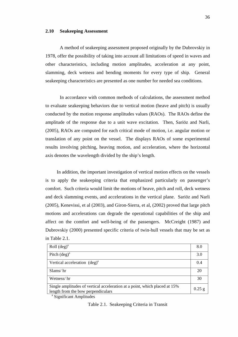
36
2.10 Seakeeping Assessment
A method of seakeeping assessment proposed originally by the Dubrovskiy in
1978, offer the possibility of taking into account all limitations of speed in waves and
other characteristics, including motion amplitudes, acceleration at any point,
slamming, deck wetness and bending moments for every type of ship. General
seakeeping characteristics are presented as one number for needed sea conditions.
In accordance with common methods of calculations, the assessment method
to evaluate seakeeping behaviors due to vertical motion (heave and pitch) is usually
conducted by the motion response amplitudes values (RAOs). The RAOs define the
amplitude of the response due to a unit wave excitation. Then, Sariöz and Narli,
(2005), RAOs are computed for each critical mode of motion, i.e. angular motion or
translation of any point on the vessel. The displays RAOs of some experimental
results involving pitching, heaving motion, and acceleration, where the horizontal
axis denotes the wavelength divided by the ship’s length.
In addition, the important investigation of vertical motion effects on the vessels
is to apply the seakeeping criteria that emphasized particularly on passenger’s
comfort. Such criteria would limit the motions of heave, pitch and roll, deck wetness
and deck slamming events, and accelerations in the vertical plane. Sariöz and Narli
(2005), Kenevissi, et al (2003), and Giron-Sierra, et al, (2002) proved that large pitch
motions and accelerations can degrade the operational capabilities of the ship and
affect on the comfort and well-being of the passengers. McCreight (1987) and
Dubrovskiy (2000) presented specific criteria of twin-hull vessels that may be set as
in Table 2.1.
Roll (deg)a 8.0
Pitch (deg)a 3.0
Vertical acceleration (deg)a 0.4
Slams/ hr 20
Wetness/ hr 30
Single amplitudes of vertical acceleration at a point, which placed at 15% length from the bow perpendiculars 0.25 g
a Significant Amplitudes
Table 2.1. Seakeeping Criteria in Transit
CHAPTER 3
APPROACH
3.1 General
This chapter puts emphasis on the evaluation of modified design hull form of
vessel to minimize the magnitude of vertical motions (pitch and heave motions) and
maintain the seakeeping quality. The genetic mutation of hull form design was taken
originally from SWATH and conventional Catamaran hull forms (has been done by
previous student). The flexible advantage of vessel is able to be operated in variable
range of draught operation i.e. shallow draught and deep draught at regular head sea
with different wavelengths. The design is readily adaptable to other applications
such as passenger vessel, geophysical research, and explorations. The over riding
design goal is good seakeeping, both dead-in-the-water and underway.
Furthermore, the detail investigations Semi-SWATH vessel performance
especially due to vertical motion at high-speed in head sea waves are presented.
Since the Semi-SWATH still has low stiffness (pitch restoring force) than the mono-
hull vessels, it result the large pitch motion, which is susceptible to trim changes in
waves. Consequently, it may cause deck wetness and makes the vessel unstable or
discomfort. While the attached pitch stabilization design (anti-pitching fins) with the
variation angle of attacks relative to the hull on the vessel can increase the vessel’s
stiffness by providing additional damping is a main consideration.
38
In order to obtain a good prediction of Semi-SWATH vessel performance in
step of time, the Time Domain Simulation is used to investigate the motion response
of Semi-SWATH vessels traveling in head seas. In addition, the development of
mathematical modelling comprising of coupled heave and pitch motion associated
with pitch stabilization is enough to identify the vessel behaviors and ensure
particularly the pitch stability in real-time simulation. However, an application of
ride control motion using conventional PID controller on the controllable stern fins
has to take into main consideration to the dynamics of Semi-SWATH motions in
which the vessel operates. The main advantage of the ride control system
development is able to adapt to every changing environment due to principal
disturbances acting on the Semi-SWATH (forces and moments generated by the
waves).
Finally, the validation of theoretical simulation will be confirmed by
experimental model test in regular head sea waves at Towing Tank of Marine
Technology Laboratory, Universiti Teknologi Malaysia.
3.2 Framework of Study
The framework of study is divided into seven phases. Explanation of each
phase is summarized as follows.
• Problem Identification
The first phase of the research is to encourage on the modified twin-hull
vessel design, which lead to reduction of magnitude vertical motion when traveling
in head seaway at high-forward speed. As mentioned in the previous chapter, this is
the most critical operation condition for twin-hull particularly Semi-SWATH vessel,
where the vessels is usually excited to large pitch motion.
• Time Domain Simulation approach
The second phase of the research is to discuss the Time Domain Simulation
approach as a tool to describe the seakeeping performance of the Semi-SWATH
vessel in head seas at high-speed. This involves the discussion of the equations of
motion and also the assumptions taken into account in the mathematical model.
39
• Validation of the Simulation Program
The third phase is to validate the simulation program results, which
conducted by the experimental Semi-SWATH model of 2.31m length carried out in
Towing Tank at Marine Technology Laboratory, Universiti Teknologi Malaysia. In
this phase is to present the validation between simulation and experiment prediction
results in a comprehensive way.
• Parametric Study
The fourth phase is to conduct parametric study. The importance of this part
is to investigate the effect of attached fin stabilizer on fore and aft body to the
vertical motion especially pitch motion in waves. The main parameter inherent to
this investigation is determined the controllable stern fin’s angle accurately to
minimize the pitch angle of vessel. Then, parametric study is carried out on the
Semi-SWATH vessel for two draught conditions with different speeds both
simulations and experiments. For the detail of this parametric study can be seen in
Table 3.1 and 3.2. It defined the comparison between simulations and experiments
correspondingly.
• Investigation of the controller scheme of the fin stabilizer on the vessel
performances
The fifth phase of the research is to investigate control scheme of fin
stabilizer as the fixed fins and controllable fins. In this phase, divided in two parts as
follows;
a) Fin with constant inclined angle relative the main hull body
This case means that the stabilizer fin is adjusted manually to have an
inclined angle relative to the ship body. The total lift on the ship is then
due to the resultant of angle of attack of incident flow to the body and the
inclined angle of fin. This technique can be applied to adjust the trim
condition of Semi-SWATH vessel advancing in waves with initial trim by
bow or stern.
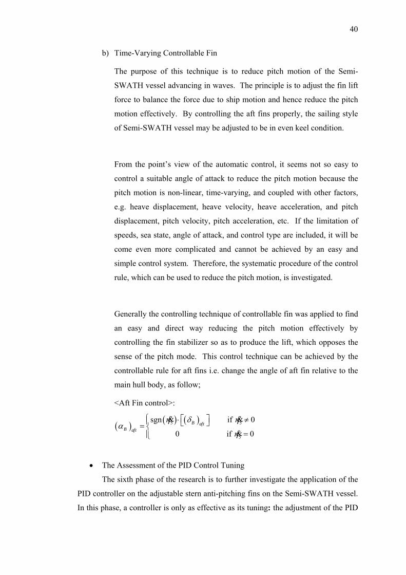
40
b) Time-Varying Controllable Fin
The purpose of this technique is to reduce pitch motion of the Semi-
SWATH vessel advancing in waves. The principle is to adjust the fin lift
force to balance the force due to ship motion and hence reduce the pitch
motion effectively. By controlling the aft fins properly, the sailing style
of Semi-SWATH vessel may be adjusted to be in even keel condition.
From the point’s view of the automatic control, it seems not so easy to
control a suitable angle of attack to reduce the pitch motion because the
pitch motion is non-linear, time-varying, and coupled with other factors,
e.g. heave displacement, heave velocity, heave acceleration, and pitch
displacement, pitch velocity, pitch acceleration, etc. If the limitation of
speeds, sea state, angle of attack, and control type are included, it will be
come even more complicated and cannot be achieved by an easy and
simple control system. Therefore, the systematic procedure of the control
rule, which can be used to reduce the pitch motion, is investigated.
Generally the controlling technique of controllable fin was applied to find
an easy and direct way reducing the pitch motion effectively by
controlling the fin stabilizer so as to produce the lift, which opposes the
sense of the pitch mode. This control technique can be achieved by the
controllable rule for aft fins i.e. change the angle of aft fin relative to the
main hull body, as follow;
<Aft Fin control>:
( ) ( ) ( )5 5
5
sgn if 0
0 if 0B aft
B aft
η δ ηα
η
⎧ ⎡ ⎤⋅ ≠⎪ ⎣ ⎦= ⎨=⎪⎩
& &
&
• The Assessment of the PID Control Tuning
The sixth phase of the research is to further investigate the application of the
PID controller on the adjustable stern anti-pitching fins on the Semi-SWATH vessel.
In this phase, a controller is only as effective as its tuning: the adjustment of the PID
41
settings relative to the process parameters to optimize load and set-point response.
Where, controller tuning involves the selection of the best values of kc, Ti and TD.
Furthermore, in order to obtain initial controller gain parameters of PID (Kp,
Ki, and Kd are the proportional, integral, and derivative gains, respectively), the
Astrom-Hagglund method based on a relay feedback controller is carried out to attain
the critical period of waveform oscillation (Tc) and critical gain (Kc).
• Evaluation of the Seakeeping Performance
The seventh phase is to present the evaluation of seakeeping performance in
all ship conditions considerably. An assessment of seakeeping characteristic
inherently produces large volume of data. Therefore, it is often necessary to select
certain parameter of the vessel for the purposes of design evaluation. The governing
criteria may vary greatly with differing vessel type and application. Moreover, they
must be appropriately selected based on the intended utilization of the design.
During simulations and experiment, the ship model without and attached fin
stabilizers incorporated with the PID controller put as a focus mainly on attenuation
of the pitch and heave position motion responses. In this thesis, the identified
seakeeping performance will be evaluated based on Response Amplitude Operators
(RAOs). For that reason, the two parameters were selected to investigate seakeeping
performances that were measured, as follows;
1. Significant heave amplitude
2. Significant pitch amplitude
3.3 Choosing a Systematic Procedure
The main reason to choose a systematic procedure is to ensure that an
objective design of the Semi-SWATH vessel development can be achieved properly.
These choosing systematic procedures will guideline for the vessel that will provide
a better seakeeping quality.
42
The adopted systematic procedure to implement the frame work of study is
divided into three main parts. There are the selection of parameters, parametric study,
and evaluation of the motion criteria in term of RAOs. The descriptions of the main
aspect in the simulation procedure are shown in the following sections.
3.3.1 Selection of Parameters
The parameters involve in the study are categorized into three groups, namely:
environmental parameters, vessel geometry, loading condition and operation
parameters.
• Environmental Parameters
The environmental parameters represent the external forces acting on the
vessel. Generally, wave, current, and wind are the main components usually
considered in the seakeeping aspects analysis. However, only the wave forces are
interested in the present study. This is because of the wave force being the main
component due to vessel suffered some uncomfortable ride and structural damage.
The waves parameters such as wave height, wave length and wave speed are
selected in the group of environmental parameters. The motions of the model in
regular wave were measured for any interest of wavelength and wave height
correspondingly. The commonly used wave height to wavelength ratio on
experiments was 1/50 (as the recommendation of the ITTC and DTNSRDC). For a
slender Semi-SWATH hull, as the present one, ship responses are assumed to be
linear for wave steepness of 1/50 or less. In addition, the range of wavelengths
covered in the experiments was restricted to 0.5 to 2.5 times the ship’s length. It
expected the peak value of Response Amplitude Operators point at certain frequency
as closed as the natural ship frequency nω both of heaving and pitching will be
achieved.
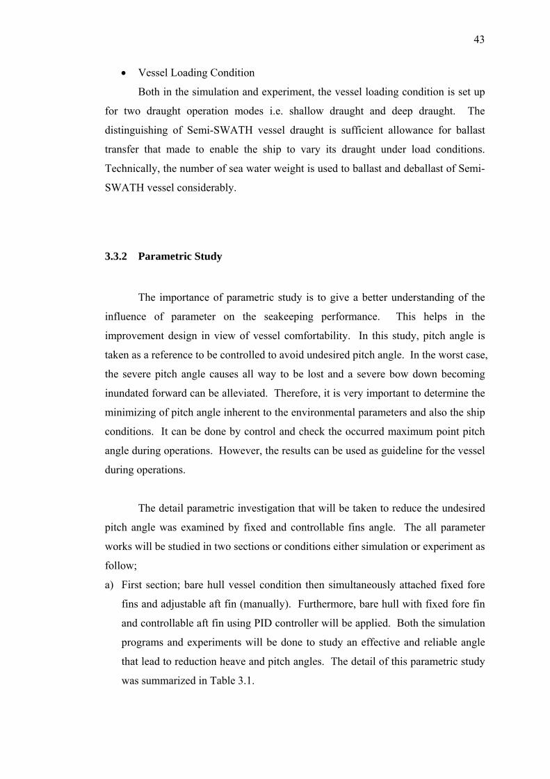
43
• Vessel Loading Condition
Both in the simulation and experiment, the vessel loading condition is set up
for two draught operation modes i.e. shallow draught and deep draught. The
distinguishing of Semi-SWATH vessel draught is sufficient allowance for ballast
transfer that made to enable the ship to vary its draught under load conditions.
Technically, the number of sea water weight is used to ballast and deballast of Semi-
SWATH vessel considerably.
3.3.2 Parametric Study
The importance of parametric study is to give a better understanding of the
influence of parameter on the seakeeping performance. This helps in the
improvement design in view of vessel comfortability. In this study, pitch angle is
taken as a reference to be controlled to avoid undesired pitch angle. In the worst case,
the severe pitch angle causes all way to be lost and a severe bow down becoming
inundated forward can be alleviated. Therefore, it is very important to determine the
minimizing of pitch angle inherent to the environmental parameters and also the ship
conditions. It can be done by control and check the occurred maximum point pitch
angle during operations. However, the results can be used as guideline for the vessel
during operations.
The detail parametric investigation that will be taken to reduce the undesired
pitch angle was examined by fixed and controllable fins angle. The all parameter
works will be studied in two sections or conditions either simulation or experiment as
follow;
a) First section; bare hull vessel condition then simultaneously attached fixed fore
fins and adjustable aft fin (manually). Furthermore, bare hull with fixed fore fin
and controllable aft fin using PID controller will be applied. Both the simulation
programs and experiments will be done to study an effective and reliable angle
that lead to reduction heave and pitch angles. The detail of this parametric study
was summarized in Table 3.1.
44
b) Second section; bare hull vessel after attached fixed fore fins and controllable aft
fins (automatically). In this case, only the simulation program incorporated with
the conventional PID controller will be studied properly. The main goal of the
second section is to achieve the pitch angle as minimum as possible with consider
the some aspects design such less resistance and passenger’s comfortability. The
detail of second section of parametric study can be seen in Table 3.1.
On the second section of parametric work will involve some chosen
controller gain parameters of PID (Kp, Ki, and Kd are the proportional, integral, and
derivative gains, respectively). The detail of this parametric study was summarized
in Table 3.2.
Table 3.1 The two sections of parameter works
Fixed Fin Angle
(Degree)
Section Case No
*S **E Vessel Condition
Fore Aft
T (M)
Vs (Knots)
1 √ √
√ -
1. Bare hull then bare with fixed fore and aft fin 2. Bare hull with fixed fore fin and con-
trollable aft fin using PID controller
15
5, 10,15 20,and
25
2.0 15
2 √ √
√ -
1. Bare hull then bare with fixed fore and aft fin 2. Bare hull with fixed fore fin and con-
trollable aft fin using PID controller
15
5, 10,15 20,and
25
1.4 20
*S for simulation **E for Experiment
Table 3.2 The parameter of PID tuning on the second section of parameter works
PID Controller Gain Fin Angle (Degree)
Case No Inner
Controller Outer
Controller
Vessel Condition Fixed
Fore (0)
Saturation of Aft fin
angle (0)
T (M)
Vs (Knots)
1 2
Kp and Kd Kp and Kd
Kp, Kd & KiKp, Kd & Ki
Bare hull with controllable aft
fins
15 15
0 to 25 0 to 25
2.0 1.4
15 20
45
3.3.3 Evaluation of Motion Response
After implementation the systematic procedures with gained the first and
second parametric studies, the results will be evaluated based on the Response
Amplitude Operators (RAOs) that plotted the each points again the ratio of sLλ . The
simple formulation of the RAOs is derived by dividing the motion amplitude by the
wave amplitude;
a
a
u motion amplitude = ξ wave ampitude
3.4 Concluding Remarks
The procedure to develop pitch improvement of Semi-SWATH vessel
operating in head seas is presented. Emphasis of the systematic procedure is to
enable achieve the desired pitch angle as minimum as possible that provide some
advantages not only in view of comfortability but also in safety. This procedure
consists of seven important phases. There are: problem identification, Time Domain
Simulation approach, validation of the simulation program, parametric study, the
assessment of the PID Control Tuning, and evaluation of the Seakeeping
Performance. Both the simulation and experiments results may be the basis for the
proposed comfort and safe design guidelines operation mainly for Semi-SWATH
vessel.
CHAPTER 4
MATHEMATICAL MODEL
4.1 General
This chapter presents the formulation for the hydrodynamic forces and
moments acting on a twin-hull vessel equipped with control surfaces, and its motion
response in step of time-domain. This formulation was developed to predict the ship
motions using strip theory. Korvin-Kroukovsky and Jacobs (1957) presented the
original strip theory especially suitable for numerical computations of heave and
pitch motions in head waves. A numerical study using a computer program based on
this formulation is also included to investigate the accuracy of the program.
The main objective of the chapter is to establish a backbone of a numerical
tool for the mathematical modeling of a ship and control surfaces in step of time-
domain with a reasonable accuracy. This model will provide a basis for a more
sophisticated time-domain model of the motion responses in the presence of active
control surfaces to be developed in chapter 5.
Therefore, in the following section (4.2) a re-statement of the formulation for
the hydrodynamic forces and moment (i.e. added mass, damping, and wave-
excitation) on a bare-hull is presented in the context of the two-dimensional linear
strip theory. The formulation of the forces and moment due to control surfaces is
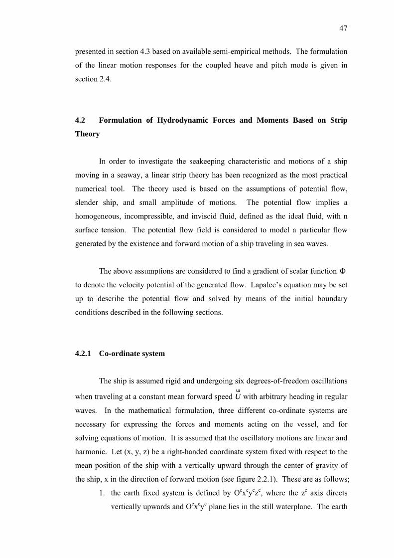
47
presented in section 4.3 based on available semi-empirical methods. The formulation
of the linear motion responses for the coupled heave and pitch mode is given in
section 2.4.
4.2 Formulation of Hydrodynamic Forces and Moments Based on Strip
Theory
In order to investigate the seakeeping characteristic and motions of a ship
moving in a seaway, a linear strip theory has been recognized as the most practical
numerical tool. The theory used is based on the assumptions of potential flow,
slender ship, and small amplitude of motions. The potential flow implies a
homogeneous, incompressible, and inviscid fluid, defined as the ideal fluid, with n
surface tension. The potential flow field is considered to model a particular flow
generated by the existence and forward motion of a ship traveling in sea waves.
The above assumptions are considered to find a gradient of scalar function Φ
to denote the velocity potential of the generated flow. Lapalce’s equation may be set
up to describe the potential flow and solved by means of the initial boundary
conditions described in the following sections.
4.2.1 Co-ordinate system
The ship is assumed rigid and undergoing six degrees-of-freedom oscillations
when traveling at a constant mean forward speed Uur
with arbitrary heading in regular
waves. In the mathematical formulation, three different co-ordinate systems are
necessary for expressing the forces and moments acting on the vessel, and for
solving equations of motion. It is assumed that the oscillatory motions are linear and
harmonic. Let (x, y, z) be a right-handed coordinate system fixed with respect to the
mean position of the ship with a vertically upward through the center of gravity of
the ship, x in the direction of forward motion (see figure 2.2.1). These are as follows;
1. the earth fixed system is defined by Oexeyeze, where the ze axis directs
vertically upwards and Oexeye plane lies in the still waterplane. The earth
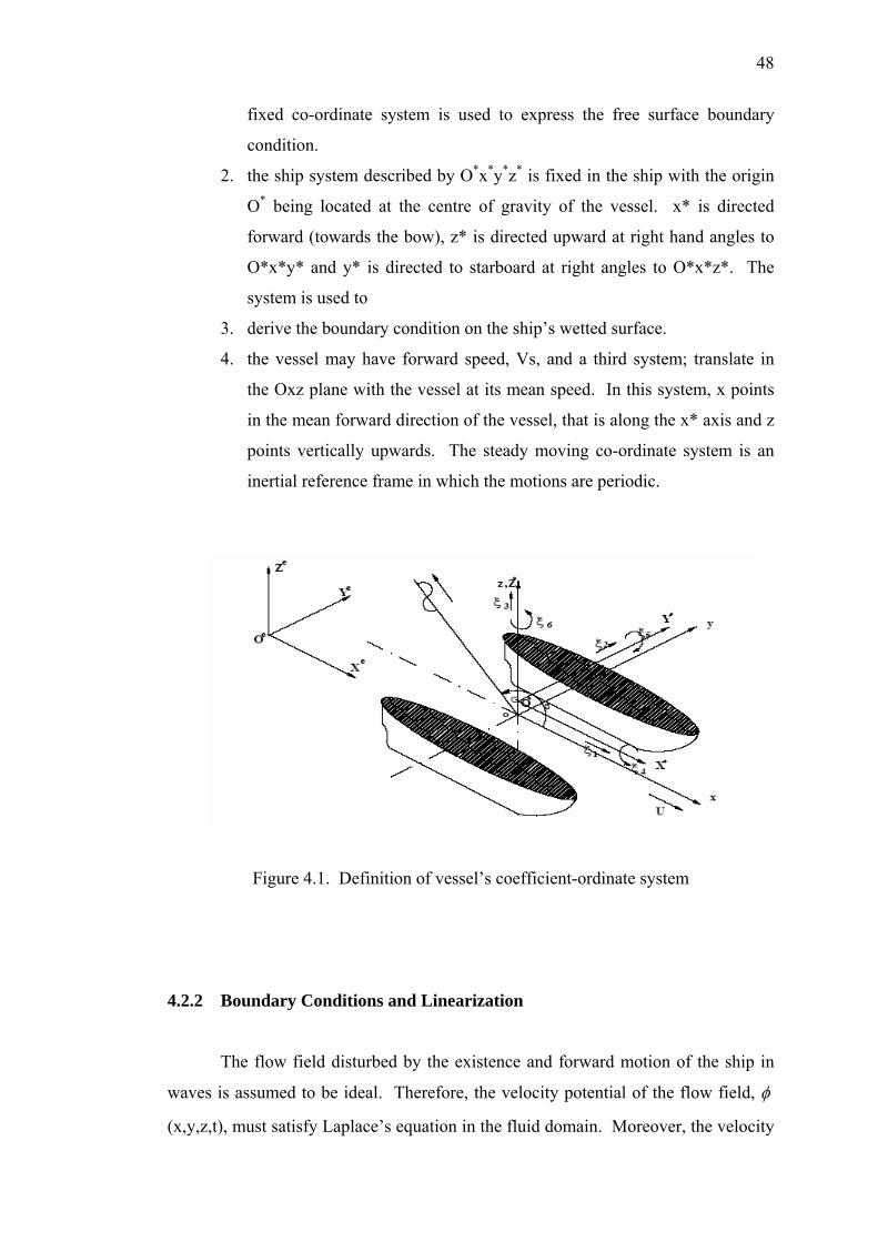
48
fixed co-ordinate system is used to express the free surface boundary
condition.
2. the ship system described by O*x*y*z* is fixed in the ship with the origin
O* being located at the centre of gravity of the vessel. x* is directed
forward (towards the bow), z* is directed upward at right hand angles to
O*x*y* and y* is directed to starboard at right angles to O*x*z*. The
system is used to
3. derive the boundary condition on the ship’s wetted surface.
4. the vessel may have forward speed, Vs, and a third system; translate in
the Oxz plane with the vessel at its mean speed. In this system, x points
in the mean forward direction of the vessel, that is along the x* axis and z
points vertically upwards. The steady moving co-ordinate system is an
inertial reference frame in which the motions are periodic.
Figure 4.1. Definition of vessel’s coefficient-ordinate system
4.2.2 Boundary Conditions and Linearization
The flow field disturbed by the existence and forward motion of the ship in
waves is assumed to be ideal. Therefore, the velocity potential of the flow field, φ
(x,y,z,t), must satisfy Laplace’s equation in the fluid domain. Moreover, the velocity
49
potential has to satisfy the equation of continuity in all points of the flow field except
at singular points. The boundaries enclosing the fluid domain consist of the wetted
body surface, the free surface, the seabed and a control surface at the far-field. It is
assumed that the sea is infinite in all horizontal directions and in depth. The velocity
potential must satisfy the conditions imposed by these boundaries.
• Free surface condition
On the free surface, the kinematic and dynamic boundary conditions imply
that a fluid particle at the surface always remains at the surface and the pressure on
the free surface is atmospheric and satisfies Bernoulli’s equation. Based on the
assumption of ideal fluid and neglecting the surface tension at the free surface, the
dynamic and kinematic boundary conditions can be combined on the free surface and
written assumption (Newman, 1978)
( )2 1- 2 - 0
2 zV V gt x t x∂ ∂ ∂ ∂⎛ ⎞ ⎛ ⎞Φ + ∇Φ ∇Φ+ ∇Φ∇ ∇Φ∇Φ + Φ =⎜ ⎟ ⎜ ⎟∂ ∂ ∂ ∂⎝ ⎠ ⎝ ⎠
(4.1)
at z = ζ the free surface
• Body surface condition
The kinematic body boundary condition indicates that the fluid velocity component
normal to the instant submerged body surface is equal to the velocity component of
the surface normal to itself. If V→
denotes the velocity of the flow and sV→
denotes
the local velocity of a point on the wetted body surface, therefore:
sV n = V n→ → → →⋅ ⋅ on wetted body surface, Sb (4.2)
where n→
is the unit vector.
• Sea bed condition
The sea bed boundary condition implies that the velocity component of fluid particle
normal to the seabed is zero since the seabed is assumed to be stationary. Thus
0n zφ φ∂ ∂= =
∂ ∂ on the sea bed z = -∞ (4.3)
50
• Radiation condition
In order to ensure having a unique, a radiation condition at infinity is
necessary to be considered. The far-field radiation condition signifies that the fluid
motion generated by the steady oscillatory body travels away from the body and
vanishes at infinity in all directions.
Since the boundary condition are highly non-linear, a perturbation expansion
scheme should be adopted. Furthermore by assuming that the vessel is slender, the
derivatives generated around the vessel will be small up to moderately high speeds.
Therefore, the derivatives can be expanded into a series form given by: 0 (0) 1 (1) 2 (2)D ε D + ε D + ε D + ...≅ (4.4)
where D indicates all derivatives around the vessel,
Bε = L is slenderness ratio,
B and L are the beam and the length of vessel respectively,
0,1 and 2 indicate the zeroth, first and second order respectively.
For the problem of a traveling vessel in waves, based on linearization, the
total velocity potential can be separated into three components given as:
( ) ( ) ( )~
xx,y,z,t = -V + x,y,z + x,y,z,tφ φΦ (4.5)
The first term on the right hand side of equation (4.5) is due to the forward
speed. The second term is called the steady perturbation potential due to the forward
motion of the vessel. The last term is the unsteady velocity potential due to the
incident and diffracted waves and the induced motions of the vessel in 6 degrees of
freedom.
Based on the above assumptions, the first order unsteady potential in equation
(4.3.5) can be expressed as:
6-iωt
0 7 j j1
= + + η eφ φ φ φ⎡ ⎤⎢ ⎥⎢ ⎥⎣ ⎦
∑ (4.6)
jη indicates the complex amplitude of the motion responses.
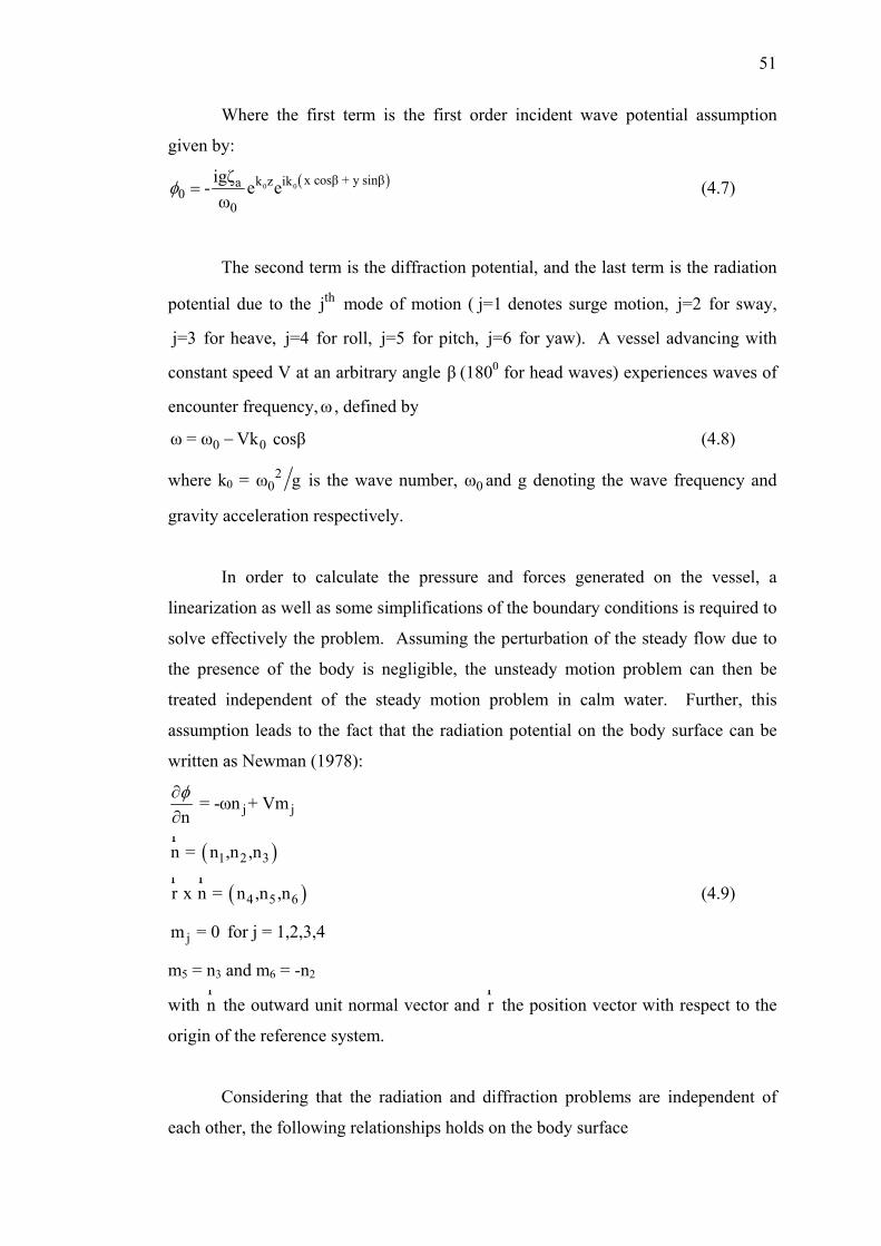
51
Where the first term is the first order incident wave potential assumption
given by:
( )0 0 x cosβ + y sinβk z ika0
0
igζ- e eω
φ = (4.7)
The second term is the diffraction potential, and the last term is the radiation
potential due to the thj mode of motion ( j=1 denotes surge motion, j=2 for sway,
j=3 for heave, j=4 for roll, j=5 for pitch, j=6 for yaw). A vessel advancing with
constant speed V at an arbitrary angle β (1800 for head waves) experiences waves of
encounter frequency,ω , defined by
0 0ω = ω Vk cosβ− (4.8)
where k0 = 20ω g is the wave number, 0ω and g denoting the wave frequency and
gravity acceleration respectively.
In order to calculate the pressure and forces generated on the vessel, a
linearization as well as some simplifications of the boundary conditions is required to
solve effectively the problem. Assuming the perturbation of the steady flow due to
the presence of the body is negligible, the unsteady motion problem can then be
treated independent of the steady motion problem in calm water. Further, this
assumption leads to the fact that the radiation potential on the body surface can be
written as Newman (1978):
j j = -ωn + Vmnφ∂∂
( )1 2 3n = n ,n ,nr
( )4 5 6r x n = n ,n ,nr r
(4.9)
jm = 0 for j = 1,2,3,4
m5 = n3 and m6 = -n2
with nr
the outward unit normal vector and rr
the position vector with respect to the
origin of the reference system.
Considering that the radiation and diffraction problems are independent of
each other, the following relationships holds on the body surface
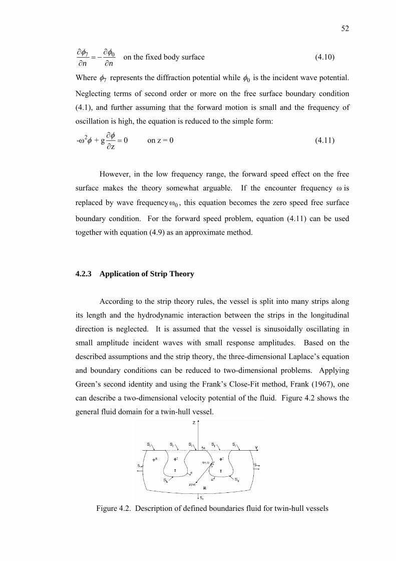
52
7 0n nφ φ∂ ∂
= −∂ ∂
on the fixed body surface (4.10)
Where 7φ represents the diffraction potential while 0φ is the incident wave potential.
Neglecting terms of second order or more on the free surface boundary condition
(4.1), and further assuming that the forward motion is small and the frequency of
oscillation is high, the equation is reduced to the simple form:
2-ω + g 0zφφ ∂=
∂ on z = 0 (4.11)
However, in the low frequency range, the forward speed effect on the free
surface makes the theory somewhat arguable. If the encounter frequency ω is
replaced by wave frequency 0ω , this equation becomes the zero speed free surface
boundary condition. For the forward speed problem, equation (4.11) can be used
together with equation (4.9) as an approximate method.
4.2.3 Application of Strip Theory
According to the strip theory rules, the vessel is split into many strips along
its length and the hydrodynamic interaction between the strips in the longitudinal
direction is neglected. It is assumed that the vessel is sinusoidally oscillating in
small amplitude incident waves with small response amplitudes. Based on the
described assumptions and the strip theory, the three-dimensional Laplace’s equation
and boundary conditions can be reduced to two-dimensional problems. Applying
Green’s second identity and using the Frank’s Close-Fit method, Frank (1967), one
can describe a two-dimensional velocity potential of the fluid. Figure 4.2 shows the
general fluid domain for a twin-hull vessel.
Figure 4.2. Description of defined boundaries fluid for twin-hull vessels
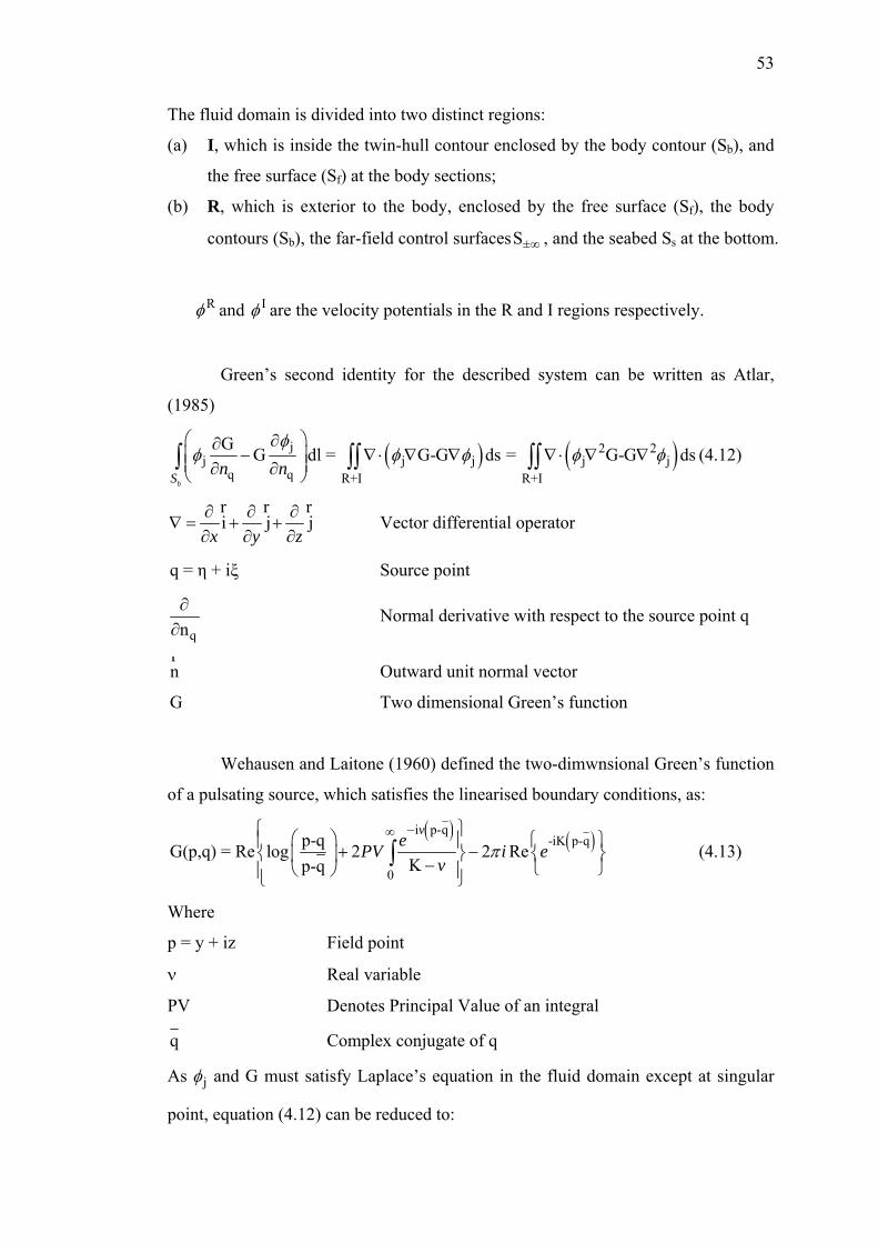
53
The fluid domain is divided into two distinct regions:
(a) I, which is inside the twin-hull contour enclosed by the body contour (Sb), and
the free surface (Sf) at the body sections;
(b) R, which is exterior to the body, enclosed by the free surface (Sf), the body
contours (Sb), the far-field control surfaces ±S ∞ , and the seabed Ss at the bottom.
Rφ and Iφ are the velocity potentials in the R and I regions respectively.
Green’s second identity for the described system can be written as Atlar,
(1985)
( ) ( )j 2 2j j j j j
q q R+I R+I
G G dl = G-G ds = G-G dsbS n n
φφ φ φ φ φ⎛ ⎞∂∂
− ∇ ⋅ ∇ ∇ ∇⋅ ∇ ∇⎜ ⎟⎜ ⎟∂ ∂⎝ ⎠∫ ∫∫ ∫∫ (4.12)
i j jx y z∂ ∂ ∂
∇ = + +∂ ∂ ∂
r r r Vector differential operator
q = η + iξ Source point
qn∂∂
Normal derivative with respect to the source point q
nr
Outward unit normal vector
G Two dimensional Green’s function
Wehausen and Laitone (1960) defined the two-dimwnsional Green’s function
of a pulsating source, which satisfies the linearised boundary conditions, as:
( ) ( )i p-q-iK p-q
0
p-qG(p,q) = Re log 2 2 ReKp-q
vePV i e
vπ
−∞⎧ ⎫⎛ ⎞ ⎧ ⎫⎪ ⎪+ −⎨ ⎬ ⎨ ⎬⎜ ⎟ − ⎩ ⎭⎝ ⎠⎪ ⎪⎩ ⎭∫ (4.13)
Where
p = y + iz Field point
ν Real variable
PV Denotes Principal Value of an integral
q Complex conjugate of q
As jφ and G must satisfy Laplace’s equation in the fluid domain except at singular
point, equation (4.12) can be reduced to:
54
b
jj
q qS
GG dl = 0n n
φφ⎛ ⎞∂∂
−⎜ ⎟⎜ ⎟∂ ∂⎝ ⎠∫ (2.14)
This equation has three different characteristics, which depend on the relative
position of the field point p to the source point q, described as follows:
(a) The field point p is inside the I region
(b) The field point, p, lies is inside the fluid domain R
(c) The field point, p, lies on the boundary contour Sb
Let the source point, q, approach the field point, when p=q, the Green’s function G
becomes singular and makes equation (4-13) invalid. This problem can be avoided
by introducing a small circle of radius ε with contour Sε and with its origin located in
R domain. Then Sb + Sε is a closed contour surrounding the fluid domain but
exterior to Sε. Defining
( ) ( ) ( )R Ij j
q q
q qn n
qφ φ
σ∂ ∂
= −∂ ∂
(4.15)
as the source strength, the velocity potential can be written in the following form.
( ) ( ) ( )b
jS
2π p q G p,q dlφ σ= ∫ (4.16)
Thus, the velocity potential is an integral of a source distribution of strength σ(q)
over the body contour and the Green’s function defined in equation (4-13).
In order to determine the source strength σ(q), the linearized body conditions (4.-9)
and (4-10) can be applied to equation (4-16). Therefore
( ) ( ) ( ) ( )
b
j
q pS
pG p,qπσ p σ q dl = 2π
n n∂∂
+∂ ∂∫
Where, the first term on the left hand side avoids the singularity problem.
The next step after calculating the source strengths is the velocity potential, which
can be determined by equation (4-16). Then, the fluid pressure, P, can be obtained
by substituting the velocity potential into unsteady bernoulli’s equation,
55
( )21P= -p gz + V2 t xφ φ⎡ ∂ ∂ ⎤⎛ ⎞∇ + −⎜ ⎟⎢ ⎥∂ ∂⎝ ⎠⎣ ⎦
(4.18)
and the fluid force, F, acting on the wetted surface, Sb, as follows:
bS
F Pnds= ∫r r
(4.19)
Where, the normal vector, nr
, directs outwards from the body surface.
4.4.4 Hydrodynamic Forces and Moments
In linear theory, the total velocity potential is the superposition of incident
velocity potential Iφ diffraction velocity potential Dφ and radiation velocity potential
Rφ therefore in order to calculate the hydrodynamic forces and moments, the
appropriate velocity potential should be substituted into the linearised Bernoulli’s
equation and then integrated over the mean wetted surface of the vessel.
If the pressure, given by equation (4.18), is expanded in a Taylor series about thr
undisturbed position of the hull and considering only terms to first order in steady
potential φ and unsteady potential ~φ the linearised time-dependent pressure on the
hull Salvesen et al. (1970) can be written as:
( )~
iωt iωt3 4 5P = -ρ i -V e - ρg η + η y + η x e
xω φ∂⎛ ⎞
⎜ ⎟∂⎝ ⎠ (4.20)
The last term gives the ordinary buoyancy restoring forces and moment. Integration
of the pressure (ignoring the buoyancy term) over the hull surface yields the
hydrodynamic forces and moment amplitudes:
b
~j j
S
H = -ρ n iω V dsx
φ∂⎛ ⎞−⎜ ⎟∂⎝ ⎠∫∫ j=1, 2, …, 6 (4.21)
56
By considering 6~
I D j jj=1
= ηφ φ φ φ+ +∑ (4.22)
the force and moment can be divided into two parts as
Hj = Fj + Gj (4.23)
Where Fj is the exciting force and moment:
( )b
-iωtj j I D
S
F ρ n iω-V dsex
φ φ∂⎛ ⎞= − +⎜ ⎟∂⎝ ⎠∫∫ (4.24)
and Gj is the force and moment due to six degrees of body motion:
b
6 6
j j k k jk kk=1 k=1S
G ρ n iω-V η ds T ηx
φ∂⎛ ⎞= − =⎜ ⎟∂⎝ ⎠∑ ∑∫∫
Here jkT denotes the hydrodynamic forces and moment in the thj direction per unit
oscillatory displacement in the thk mode:
b
6
jk j kk=1S
T ρ n iω-V dsx
φ∂⎛ ⎞= − ⎜ ⎟∂⎝ ⎠∑∫∫ (4.26)
After separating jkT into real and imaginary parts as:
2jk jk jkT ω A - iωB= (4.27)
the added mass and damping can be defined in the form
b
6
jk j k2k=1S
ρA Re n iω-V dsxω
φ− ∂⎛ ⎞= ⎜ ⎟∂⎝ ⎠∑∫∫ (4.28)
b
6
jk j kk=1S
ρB Im n iω-V dsω x
φ− ∂⎛ ⎞= ⎜ ⎟∂⎝ ⎠∑∫∫ (4.29)
4.3 Modelling of Fin Effect
The forces and moments generated by the presence of fin stabilizers can be
represented in term of the motion equation coefficients and external forces terms as,
ff f f f f.. . keF = A +M η +B η+C η- F +Fji ij ij ij ij iij
⎡ ⎤⎡ ⎤∑ ⎢ ⎥⎣ ⎦ ⎣ ⎦ (4.30)
57
where superscript is associated with fins, e the wave-excitation, and k the control
forces due to the activation of the fins.
The forces and moments on n pairs of fins, can be assumed to have three component,
which are associated with the lift, Lin drag, Din and virtual inertia effects, Iin ,of
the surrounding flow. Therefore,
f NF = L +D +Ii in in inn=1
⎡ ⎤∑ ⎣ ⎦ (4.31)
The lift component generated by the quasi-static pitch of the hull and deflection of
the fins can be written as
2ρL = V A C α+C δLαin Lδ2 (4.32)
where ρ is the fluid density, V is the fluid velocity, A is the projected fin area,
CLα is the lift coefficient of the fin due to hull pitch angel α , the fin being
considered fixed to the hull, and CLδ is the lift coefficient due to control deflection
δ with respect to the hull. The values of the lift coefficients based on the slender
body theory for a single fin attached to a circular hull, Caldeira-Saraiva and Clarke
(1988), are given by
[ ]Lα LαW(B) W(B) WC = K +K C⎡ ⎤⎣ ⎦ (4.33)
[ ]LαLδ W(B) W(B) WC = k +k C⎡ ⎤⎣ ⎦ (4.34)
Where, the subscripts B and W represent Body (or hull) and Wing (or fin)
respectively. The fin-hull interaction factors, K for a fixed fin and k for an
activating fin, are devined by the following relationships Kuerti et al (1952),
W(B) W(B)
21K +K 1 22
a as s
⎡ ⎤= + +⎢ ⎥⎣ ⎦ (4.35)
And
W(B) W(B)
3 -3 -1 12 2 2 2
22 1k +k = λ -λ +7λ -7λ
2π(λ-1)⎧ ⎡ ⎤ +⎨ ⎢ ⎥⎣ ⎦⎩
(4.36)
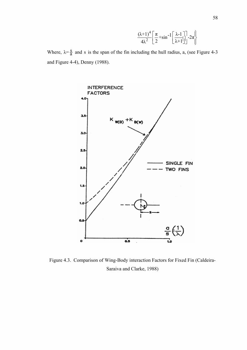
58
4
2(λ+1) π λ-1-1+sin -2π
2 λ+14λ
⎫⎡ ⎤ ⎪⎡ ⎤⎬⎢ ⎥⎢ ⎥⎣ ⎦⎣ ⎦ ⎪⎭
Where, sλ= a and s is the span of the fin including the hull radius, a, (see Figure 4-3
and Figure 4-4), Denny (1988).
Figure 4.3. Comparison of Wing-Body interaction Factors for Fixed Fin (Caldeira-
Saraiva and Clarke, 1988)
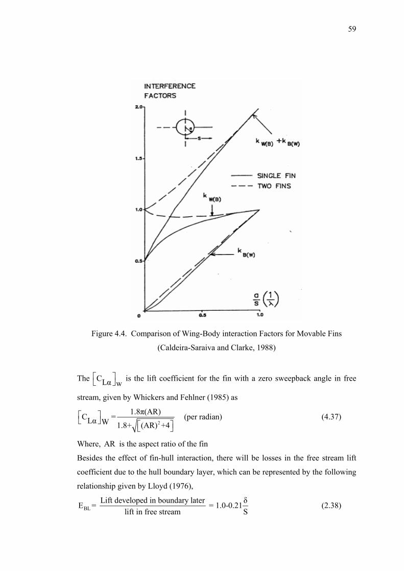
59
Figure 4.4. Comparison of Wing-Body interaction Factors for Movable Fins
(Caldeira-Saraiva and Clarke, 1988)
The CLα w⎡ ⎤⎣ ⎦ is the lift coefficient for the fin with a zero sweepback angle in free
stream, given by Whickers and Fehlner (1985) as
2
1.8π(AR)C = (per radian)Lα W 1.8+ (AR) +4⎡ ⎤⎣ ⎦ ⎡ ⎤⎣ ⎦
(4.37)
Where, AR is the aspect ratio of the fin
Besides the effect of fin-hull interaction, there will be losses in the free stream lift
coefficient due to the hull boundary layer, which can be represented by the following
relationship given by Lloyd (1976),
BLLift developed in boundary later δE = = 1.0-0.21
lift in free stream S (2.38)
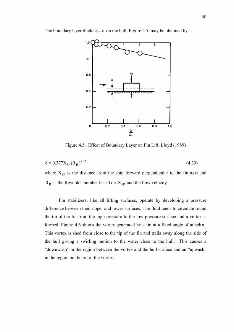
60
The boundary layer thickness δ on the hull, Figure 2.5, may be obtained by
Figure 4.5. Effect of Boundary Layer on Fin Lift, Lloyd (1989)
FP-0.2δ = 0.377X (R )n (4.39)
where FPX is the distance from the ship forward perpendicular to the fin axis and
Rn is the Reynolds number based on FPX and the flow velocity .
Fin stabilizers, like all lifting surfaces, operate by developing a pressure
difference between their upper and lower surfaces. The fluid tends to circulate round
the tip of the fin from the high pressure to the low-pressure surface and a vortex is
formed. Figure 4.6 shows the vortex generated by a fin at a fixed angle of attackα .
This vortex is shed from close to the tip of the fin and trails away along the side of
the hull giving a swirling motion to the water close to the hull. This causes a
“downwash” in the region between the vortex and the hull surface and an “upwash”
in the region out board of the vortex.
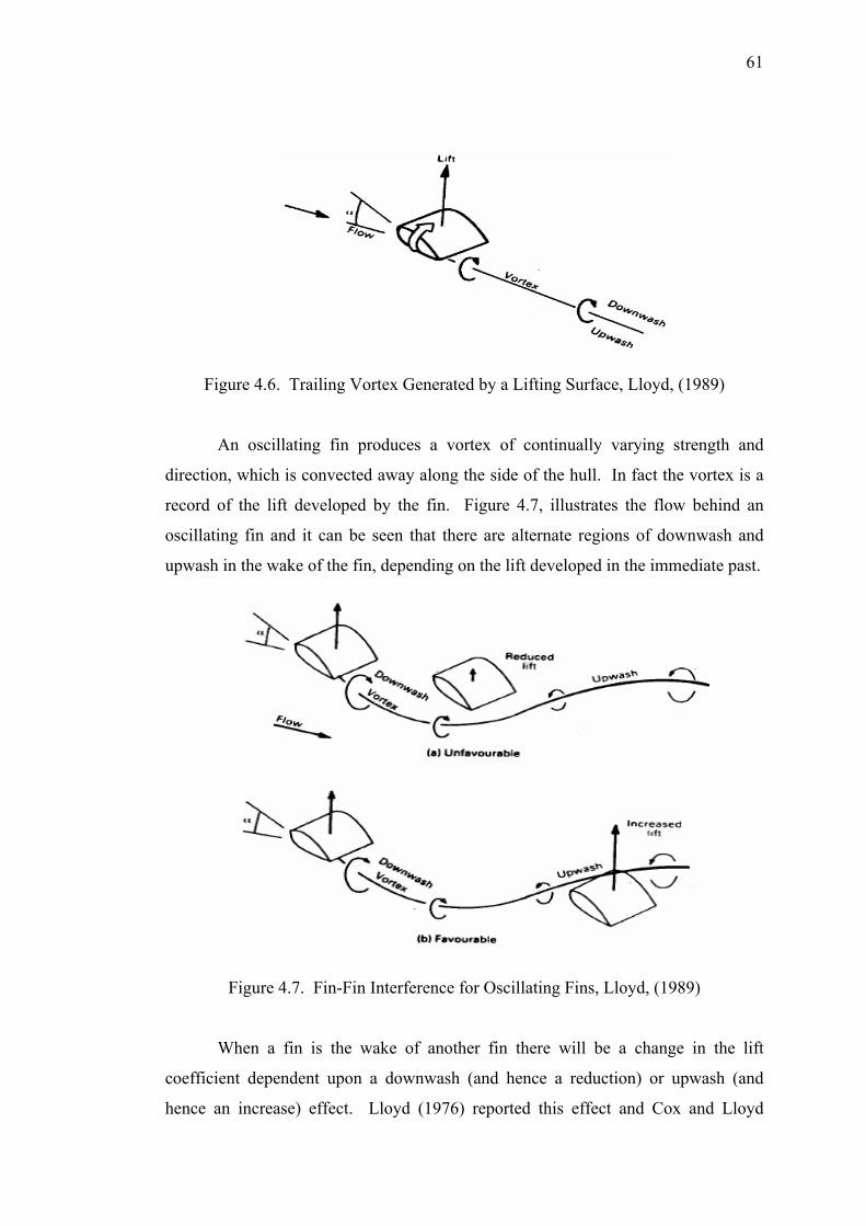
61
Figure 4.6. Trailing Vortex Generated by a Lifting Surface, Lloyd, (1989)
An oscillating fin produces a vortex of continually varying strength and
direction, which is convected away along the side of the hull. In fact the vortex is a
record of the lift developed by the fin. Figure 4.7, illustrates the flow behind an
oscillating fin and it can be seen that there are alternate regions of downwash and
upwash in the wake of the fin, depending on the lift developed in the immediate past.
Figure 4.7. Fin-Fin Interference for Oscillating Fins, Lloyd, (1989)
When a fin is the wake of another fin there will be a change in the lift
coefficient dependent upon a downwash (and hence a reduction) or upwash (and
hence an increase) effect. Lloyd (1976) reported this effect and Cox and Lloyd
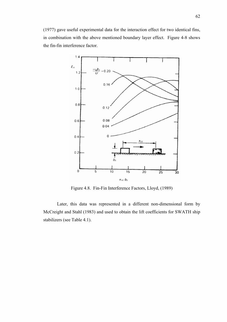
62
(1977) gave useful experimental data for the interaction effect for two identical fins,
in combination with the above mentioned boundary layer effect. Figure 4-8 shows
the fin-fin interference factor.
Figure 4.8. Fin-Fin Interference Factors, Lloyd, (1989)
Later, this data was represented in a different non-dimensional form by
McCreight and Stahl (1983) and used to obtain the lift coefficients for SWATH ship
stabilizers (see Table 4.1).
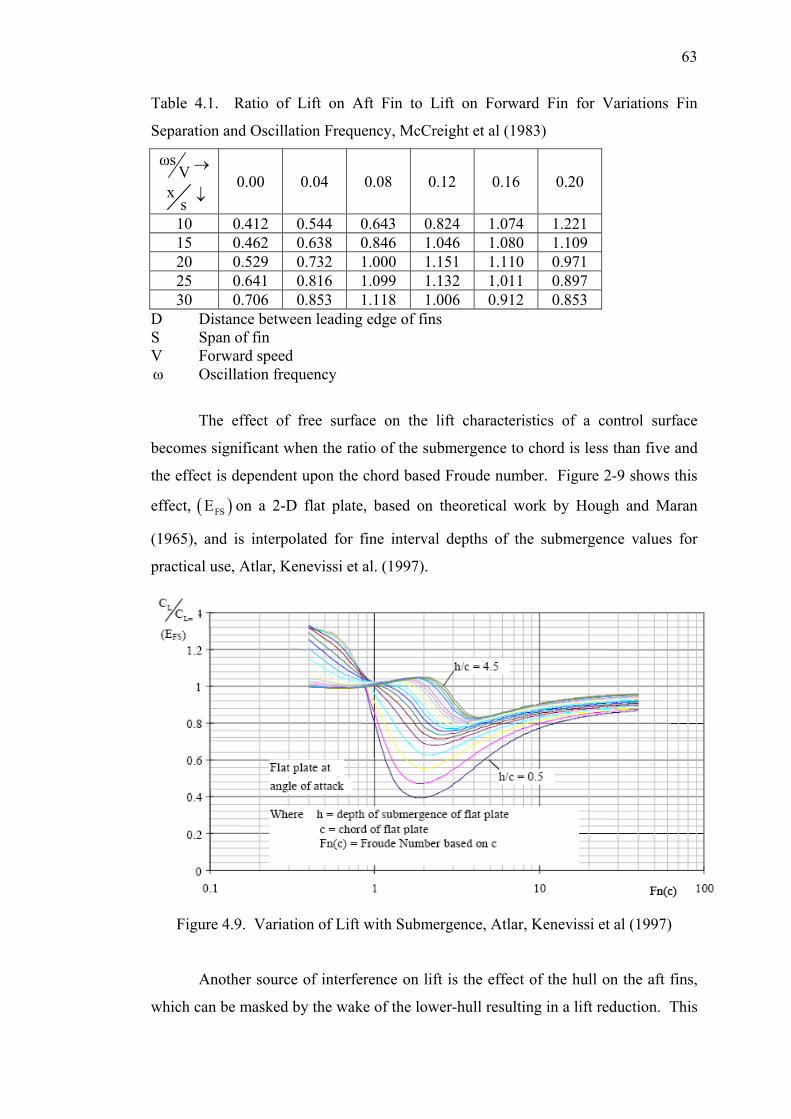
63
Table 4.1. Ratio of Lift on Aft Fin to Lift on Forward Fin for Variations Fin
Separation and Oscillation Frequency, McCreight et al (1983)
ωsV →
xs ↓
0.00 0.04 0.08 0.12 0.16 0.20
10 0.412 0.544 0.643 0.824 1.074 1.221 15 0.462 0.638 0.846 1.046 1.080 1.109 20 0.529 0.732 1.000 1.151 1.110 0.971 25 0.641 0.816 1.099 1.132 1.011 0.897 30 0.706 0.853 1.118 1.006 0.912 0.853
D Distance between leading edge of fins S Span of fin V Forward speed ω Oscillation frequency
The effect of free surface on the lift characteristics of a control surface
becomes significant when the ratio of the submergence to chord is less than five and
the effect is dependent upon the chord based Froude number. Figure 2-9 shows this
effect, ( )FSE on a 2-D flat plate, based on theoretical work by Hough and Maran
(1965), and is interpolated for fine interval depths of the submergence values for
practical use, Atlar, Kenevissi et al. (1997).
Figure 4.9. Variation of Lift with Submergence, Atlar, Kenevissi et al (1997)
Another source of interference on lift is the effect of the hull on the aft fins,
which can be masked by the wake of the lower-hull resulting in a lift reduction. This
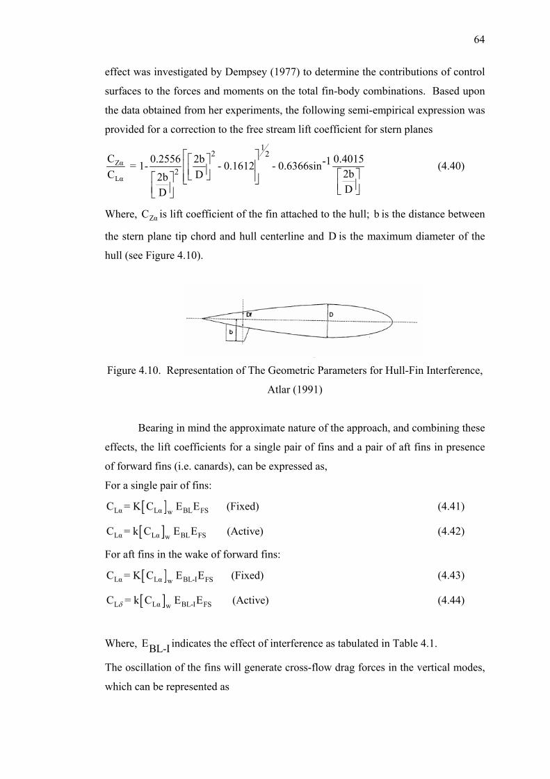
64
effect was investigated by Dempsey (1977) to determine the contributions of control
surfaces to the forces and moments on the total fin-body combinations. Based upon
the data obtained from her experiments, the following semi-empirical expression was
provided for a correction to the free stream lift coefficient for stern planes
Zα
Lα
12 2
2C 0.2556 2b 0.4015-1 = 1- - 0.1612 - 0.6366sin
2bC D2bDD
⎡ ⎤⎡ ⎤⎢ ⎥⎢ ⎥ ⎡ ⎤⎣ ⎦⎢ ⎥⎡ ⎤ ⎣ ⎦ ⎢ ⎥⎢ ⎥ ⎣ ⎦⎣ ⎦
(4.40)
Where, ZαC is lift coefficient of the fin attached to the hull; b is the distance between
the stern plane tip chord and hull centerline and D is the maximum diameter of the
hull (see Figure 4.10).
Figure 4.10. Representation of The Geometric Parameters for Hull-Fin Interference,
Atlar (1991)
Bearing in mind the approximate nature of the approach, and combining these
effects, the lift coefficients for a single pair of fins and a pair of aft fins in presence
of forward fins (i.e. canards), can be expressed as,
For a single pair of fins:
[ ]Lα Lα BL FSwC = K C E E (Fixed) (4.41)
[ ]Lα Lα BL FSwC = k C E E (Active) (4.42)
For aft fins in the wake of forward fins:
[ ]Lα Lα BL-I FSwC = K C E E (Fixed) (4.43)
[ ]Lα BL-IL FSwC = k C E E (Active)δ (4.44)
Where, EBL-I indicates the effect of interference as tabulated in Table 4.1.
The oscillation of the fins will generate cross-flow drag forces in the vertical modes,
which can be represented as
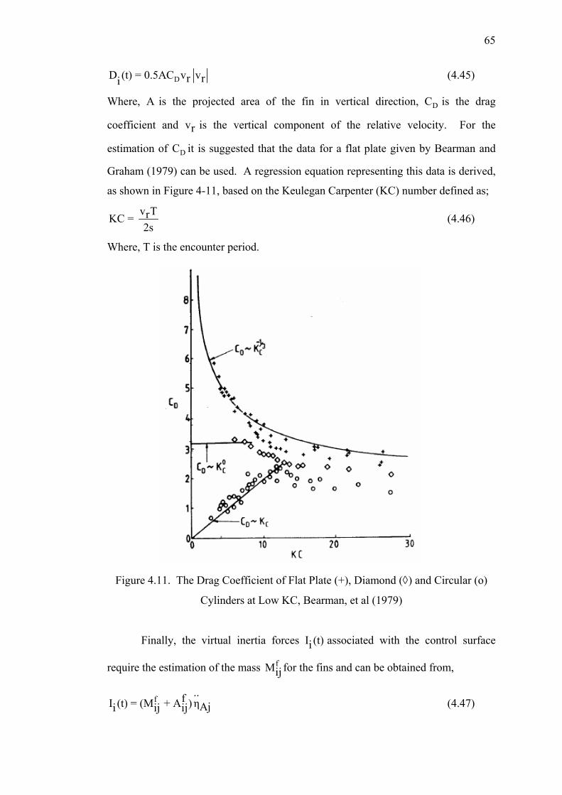
65
DD (t) = 0.5AC v vr ri (4.45)
Where, A is the projected area of the fin in vertical direction, DC is the drag
coefficient and vr is the vertical component of the relative velocity. For the
estimation of DC it is suggested that the data for a flat plate given by Bearman and
Graham (1979) can be used. A regression equation representing this data is derived,
as shown in Figure 4-11, based on the Keulegan Carpenter (KC) number defined as;
v TrKC = 2s
(4.46)
Where, T is the encounter period.
Figure 4.11. The Drag Coefficient of Flat Plate (+), Diamond (◊) and Circular (o)
Cylinders at Low KC, Bearman, et al (1979)
Finally, the virtual inertia forces I (t)i associated with the control surface
require the estimation of the mass fMij for the fins and can be obtained from,
f..fI (t) = (M + A )ηAji ij ij (4.47)
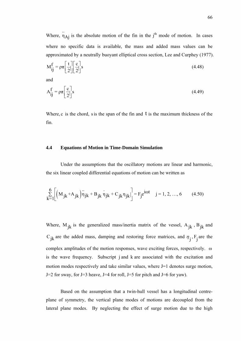
66
Where, ..ηAj is the absolute motion of the fin in the jth mode of motion. In cases
where no specific data is available, the mass and added mass values can be
approximated by a neutrally buoyant elliptical cross section, Lee and Curphey (1977).
t cfM = ρπ sij 2 2⎡ ⎤ ⎡ ⎤⎢ ⎥ ⎢ ⎥⎣ ⎦ ⎣ ⎦
(4.48)
and
cfA = ρπ sij 2⎡ ⎤⎢ ⎥⎣ ⎦
(4.49)
Where, c is the chord, s is the span of the fin and t is the maximum thickness of the
fin.
4.4 Equations of Motion in Time-Domain Simulation
Under the assumptions that the oscillatory motions are linear and harmonic,
the six linear coupled differential equations of motion can be written as
( ) .. .6 iωtM +A η + B η + C η = F ejk jkjk jk jk jk jk jk=1⎡ ⎤
∑ ⎢ ⎥⎣ ⎦
j = 1, 2, …, 6 (4.50)
Where, M jk is the generalized mass/inertia matrix of the vessel, A jk , Bjk and
Cjk are the added mass, damping and restoring force matrices, and jη , Fj are the
complex amplitudes of the motion responses, wave exciting forces, respectively. ω
is the wave frequency. Subscript j and k are associated with the excitation and
motion modes respectively and take similar values, where J=1 denotes surge motion,
J=2 for sway, for J=3 heave, J=4 for roll, J=5 for pitch and J=6 for yaw).
Based on the assumption that a twin-hull vessel has a longitudinal centre-
plane of symmetry, the vertical plane modes of motions are decoupled from the
lateral plane modes. By neglecting the effect of surge motion due to the high
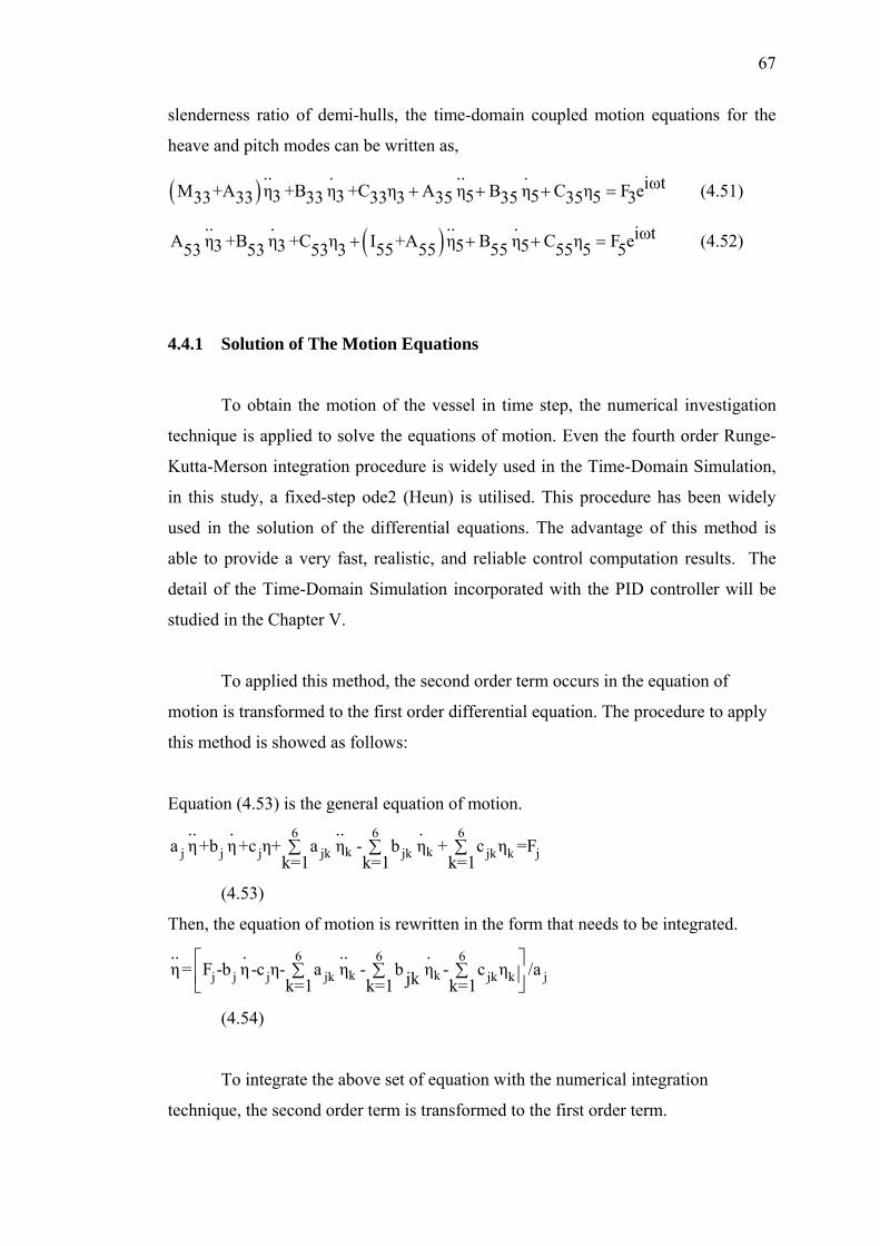
67
slenderness ratio of demi-hulls, the time-domain coupled motion equations for the
heave and pitch modes can be written as,
( ).. . .. . iωtM +A η +B η +C η A η B η C η F e3 3 5 5 533 33 33 33 3 35 35 35 3+ + + = (4.51)
( ).. . .. . iωtA η +B η +C η I +A η B η C η F e3 3 5 555 55 55 55 5 553 53 53 3 + + + = (4.52)
4.4.1 Solution of The Motion Equations
To obtain the motion of the vessel in time step, the numerical investigation
technique is applied to solve the equations of motion. Even the fourth order Runge-
Kutta-Merson integration procedure is widely used in the Time-Domain Simulation,
in this study, a fixed-step ode2 (Heun) is utilised. This procedure has been widely
used in the solution of the differential equations. The advantage of this method is
able to provide a very fast, realistic, and reliable control computation results. The
detail of the Time-Domain Simulation incorporated with the PID controller will be
studied in the Chapter V.
To applied this method, the second order term occurs in the equation of
motion is transformed to the first order differential equation. The procedure to apply
this method is showed as follows:
Equation (4.53) is the general equation of motion. 6 6 6
k kj j j jk jk jk k j
.. . .. .a η+b η+c η+ a η - b η + c η =F
k=1 k=1 k=1∑ ∑ ∑
(4.53)
Then, the equation of motion is rewritten in the form that needs to be integrated.
6 6 6k kj j j jk jk k j
.. . .. .η= F -b η -c η- a η - b η - c η /ajkk=1 k=1 k=1
⎡ ⎤∑ ∑ ∑⎢ ⎥⎣ ⎦
(4.54)
To integrate the above set of equation with the numerical integration
technique, the second order term is transformed to the first order term.
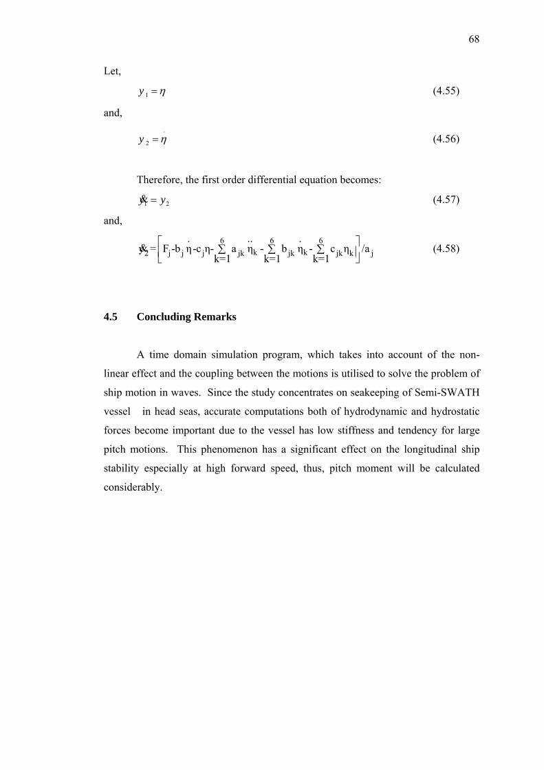
68
Let,
1y η= (4.55)
and,
.
2y η= (4.56)
Therefore, the first order differential equation becomes:
21 yy =& (4.57)
and,
6 6 6
k k2 j j j jk jk jk k j
. .. .y = F -b η -c η- a η - b η - c η /a
k=1 k=1 k=1⎡ ⎤
∑ ∑ ∑⎢ ⎥⎣ ⎦& (4.58)
4.5 Concluding Remarks
A time domain simulation program, which takes into account of the non-
linear effect and the coupling between the motions is utilised to solve the problem of
ship motion in waves. Since the study concentrates on seakeeping of Semi-SWATH
vessel in head seas, accurate computations both of hydrodynamic and hydrostatic
forces become important due to the vessel has low stiffness and tendency for large
pitch motions. This phenomenon has a significant effect on the longitudinal ship
stability especially at high forward speed, thus, pitch moment will be calculated
considerably.
CHAPTER 5
IMPROVED VESSEL RIDE PERFORMANCE
USING TIME-DOMAIN SIMULATION
5.1 General
This chapter presents the formulation and numerical applications for an
optimal strategy to improve the ride performance of Semi-SWATH vessel using
Time-Domain Simulation. To improve the robustness of the control system, the
application of conventional PID control is applied.
The PID Control is a classical control technique, its acronym of PID stands
for Proportional-Integral-Derivative. Inherent to its control law, the PID Control can
be designed not only to control a single-input single-output (SISO) controller but
also to handle multiple-input multiple-output (MIMO) systems.
The primary advantage using The PID controller is providing a robust
performance for a wide range of operating conditions. Furthermore, it is easy to
implement using analogue or digital hardware and familiar to engineers. Previously,
many researchers e.g. Caldeira, et al (1984), ware, et al (1980a), (1980b), 1981, and
1987, and Chinn, et al (1994) applied conventional optimal controller design to
improve the vertical motion response of marine vehicles.
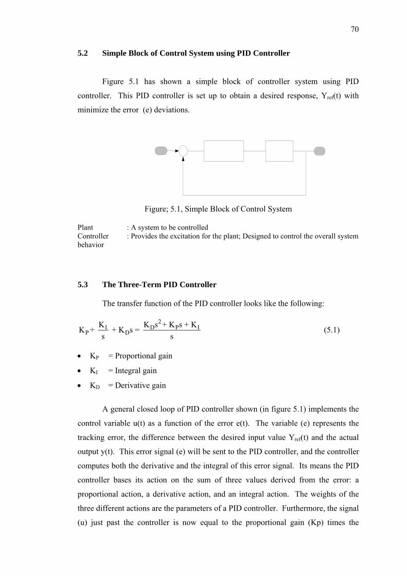
70
5.2 Simple Block of Control System using PID Controller
Figure 5.1 has shown a simple block of controller system using PID
controller. This PID controller is set up to obtain a desired response, Yref(t) with
minimize the error (e) deviations.
Figure; 5.1, Simple Block of Control System Plant : A system to be controlled Controller : Provides the excitation for the plant; Designed to control the overall system behavior 5.3 The Three-Term PID Controller
The transfer function of the PID controller looks like the following:
2I D P I
P DK K s + K s + KK + + K s = s s
(5.1)
• KP = Proportional gain
• KI = Integral gain
• KD = Derivative gain
A general closed loop of PID controller shown (in figure 5.1) implements the
control variable u(t) as a function of the error e(t). The variable (e) represents the
tracking error, the difference between the desired input value Yref(t) and the actual
output y(t). This error signal (e) will be sent to the PID controller, and the controller
computes both the derivative and the integral of this error signal. Its means the PID
controller bases its action on the sum of three values derived from the error: a
proportional action, a derivative action, and an integral action. The weights of the
three different actions are the parameters of a PID controller. Furthermore, the signal
(u) just past the controller is now equal to the proportional gain (Kp) times the
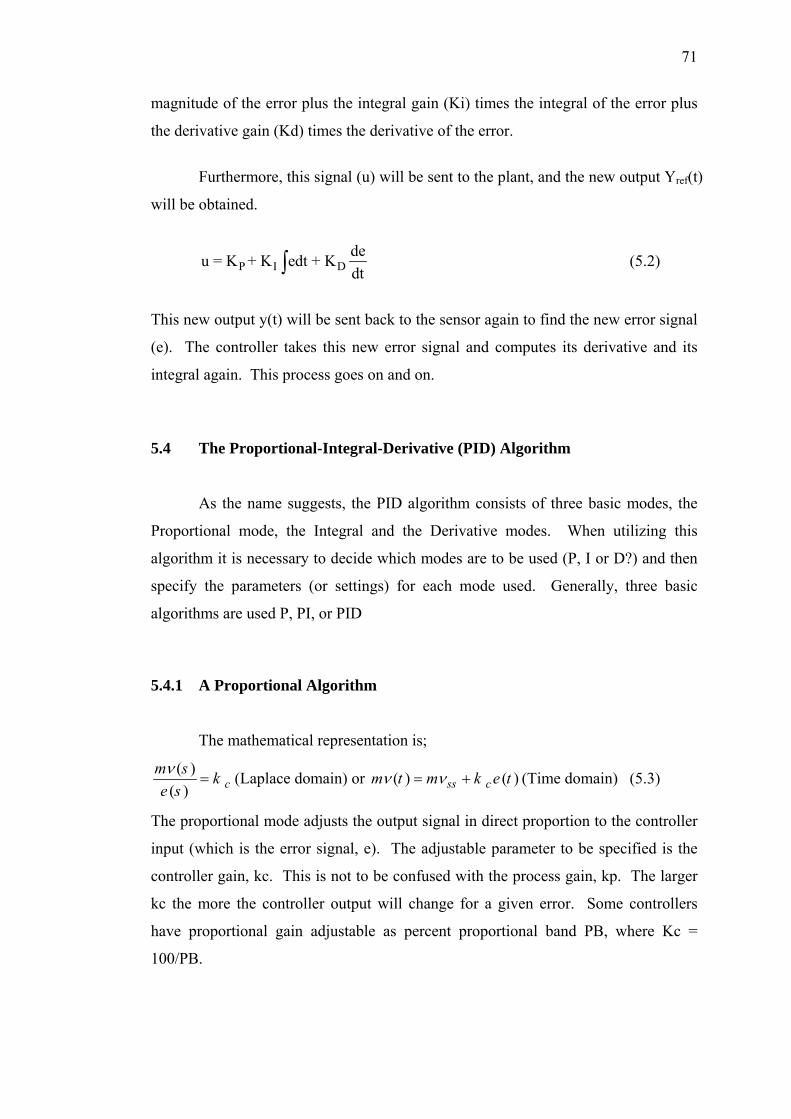
71
magnitude of the error plus the integral gain (Ki) times the integral of the error plus
the derivative gain (Kd) times the derivative of the error.
Furthermore, this signal (u) will be sent to the plant, and the new output Yref(t)
will be obtained.
P I Ddeu = K + K edt + Kdt∫ (5.2)
This new output y(t) will be sent back to the sensor again to find the new error signal
(e). The controller takes this new error signal and computes its derivative and its
integral again. This process goes on and on.
5.4 The Proportional-Integral-Derivative (PID) Algorithm
As the name suggests, the PID algorithm consists of three basic modes, the
Proportional mode, the Integral and the Derivative modes. When utilizing this
algorithm it is necessary to decide which modes are to be used (P, I or D?) and then
specify the parameters (or settings) for each mode used. Generally, three basic
algorithms are used P, PI, or PID
5.4.1 A Proportional Algorithm
The mathematical representation is;
( )( ) c
m s ke sν
= (Laplace domain) or ( ) ( )ss cm t m k e tν ν= + (Time domain) (5.3)
The proportional mode adjusts the output signal in direct proportion to the controller
input (which is the error signal, e). The adjustable parameter to be specified is the
controller gain, kc. This is not to be confused with the process gain, kp. The larger
kc the more the controller output will change for a given error. Some controllers
have proportional gain adjustable as percent proportional band PB, where Kc =
100/PB.
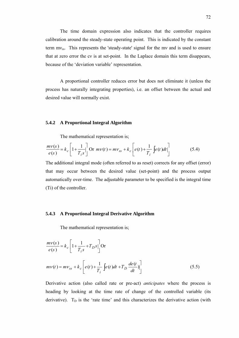
72
The time domain expression also indicates that the controller requires
calibration around the steady-state operating point. This is indicated by the constant
term mνss. This represents the 'steady-state' signal for the mν and is used to ensure
that at zero error the cν is at set-point. In the Laplace domain this term disappears,
because of the ‘deviation variable’ representation.
A proportional controller reduces error but does not eliminate it (unless the
process has naturally integrating properties), i.e. an offset between the actual and
desired value will normally exist.
5.4.2 A Proportional Integral Algorithm
The mathematical representation is;
( ) 11( ) c
i
m s ke s T sν ⎡ ⎤
= +⎢ ⎥⎣ ⎦
Or 1( ) ( ) ( )ss ci
m t m k e t e t dtT
ν ν⎡ ⎤
= + +⎢ ⎥⎣ ⎦
∫ (5.4)
The additional integral mode (often referred to as reset) corrects for any offset (error)
that may occur between the desired value (set-point) and the process output
automatically over-time. The adjustable parameter to be specified is the integral time
(Ti) of the controller.
5.4.3 A Proportional Integral Derivative Algorithm
The mathematical representation is;
( ) 11( ) c D
i
m s k T se s T sν ⎡ ⎤
= + +⎢ ⎥⎣ ⎦
Or
1 (( ) ( ) ( ) )ss c Di
de tm t m k e t e t dt TT dt
ν ν⎡ ⎤
= + + +⎢ ⎥⎣ ⎦
∫ (5.5)
Derivative action (also called rate or pre-act) anticipates where the process is
heading by looking at the time rate of change of the controlled variable (its
derivative). TD is the ‘rate time’ and this characterizes the derivative action (with
73
units of minutes). In theory derivative action should always improve dynamic
response and it does in many loops. In others, however, the problem of noisy signals
makes the use of derivative action undesirable (differentiating noisy signals can
translate into excessive mν movement). Furthermore, Derivative action depends on
the slope of the error, unlike P and I. If the error is constant derivative action has no
effect.
5.5 Controller Tuning
A controller is only as effective as its tuning: the adjustment of the PID
settings relative to the process parameters to optimize load and set-point response.
Where, controller tuning involves the selection of the best values of kc, Ti and TD (if
a PID algorithm is being used). This is often a subjective procedure and is certainly
process dependent. A number of methods have been proposed in the literature over
the last 50 years. Tuning is required when the controller is first commissioned on a
loop, and may have to be repeated if process parameters change appreciably with
time, load, set point, etc. The suggestion being a PID controller can be properly
tuned to improve the operational performance of process plant to match some
preconceived 'ideal' response profile for the closed loop system.
5.5.1 Parameter Tuning Rules for PID Controller
As written in the equation (5.1), the transfer function of a PID controller can
be modified in the following form:
11PID p di
G K T sT s
⎛ ⎞= + + +⎜ ⎟
⎝ ⎠ (5.6 )
Where pi
i
KT
K= and d
dp
KTK
= , Ti and Td are the integral time constant and the
derivative time constant, respectively.
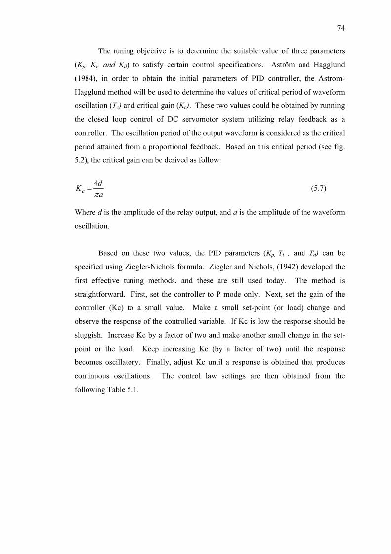
74
The tuning objective is to determine the suitable value of three parameters
(Kp, Ki, and Kd) to satisfy certain control specifications. Aström and Hagglund
(1984), in order to obtain the initial parameters of PID controller, the Astrom-
Hagglund method will be used to determine the values of critical period of waveform
oscillation (Tc) and critical gain (Kc). These two values could be obtained by running
the closed loop control of DC servomotor system utilizing relay feedback as a
controller. The oscillation period of the output waveform is considered as the critical
period attained from a proportional feedback. Based on this critical period (see fig.
5.2), the critical gain can be derived as follow:
4
cdKaπ
= (5.7)
Where d is the amplitude of the relay output, and a is the amplitude of the waveform
oscillation.
Based on these two values, the PID parameters (Kp, Ti , and Td) can be
specified using Ziegler-Nichols formula. Ziegler and Nichols, (1942) developed the
first effective tuning methods, and these are still used today. The method is
straightforward. First, set the controller to P mode only. Next, set the gain of the
controller (Kc) to a small value. Make a small set-point (or load) change and
observe the response of the controlled variable. If Kc is low the response should be
sluggish. Increase Kc by a factor of two and make another small change in the set-
point or the load. Keep increasing Kc (by a factor of two) until the response
becomes oscillatory. Finally, adjust Kc until a response is obtained that produces
continuous oscillations. The control law settings are then obtained from the
following Table 5.1.
75
Table 5.1 Ziegler-Nichols Parameter Tuning
Kp Ti Td P 0.5 Kc PI 0.45 Kc 0.85 Tc PID 0.6 Kc 0.5 Tc 0.125 Tc
Figure 5.2 The relay feedback controller 5.6 Actuator Modeling
The electromechanical dual acting on the fin stabilizer shaft system was
utilized two DC servomotors ac actuators. Output shaft of the DC servomotor is
directly connected to a series of gear reducers to initiate the fin shaft’s movement.
Based on this arrangement, the DC servomotor enables to control the shaft’s
movements directly.
5.6.1 Modeling of DC Servomotor
The dynamic model of the DC servomotor is represented as follow:
aaaaa
aa KRdtd
LV ii ω++= . (5.8)
Tm = Km. ia (5.9)
76
Tm – TL = Jm (dω/dt)+Bm(dθ/dt) (5.10)
By using LaPlace Operator s = d/dt, then
ωaaaaaa KiRisLV ++= (5.11)
aaaaaa iRiLsKV .... +=− ω (5.12)
Tm - TL = Jm .s.ω +Bm.s2.ω (5.13)
θ = ω /s (5.14)
Where :
Va : Motor Voltage [V]
La : Motor Inductance [H]
ia : Motor Current [A]
Ra : Motor Resistance [Ω]
Ka : Back emf constant [mV/(rad/sec)]
ω : Motor shaft angular velocity [rad/sec]
θ : Angular displacement [rad]
Tm : Motor Torque [Nm]
Km : Torque Constant [Nm/A]
TL : Load Torque [Nm]
Jm : Motor Inertia [Nm.sec2]
For the detail of servo motor parameter used in this simulation, see Table 5.2.
The simulation control studies of the proposed PID controller are carried out in
order to investigate its effectiveness in this position control application. In these
studies, the DC servomotor as the actuator has the following important parameters as
shown in Table 5.2.
77
Table 5.2 DC servomotor parameters
Parameters Values Motor Voltage 24 V Armature Resistance 0.03 Ω Armature Inductance 0.1 mH Back emf Constant 7 mV/rpm Torque Constant 0.0674 N/A Nominal Torque 1.6 Nm Nominal Speed 3000 rpm Rotor Inertia 0.1555e-4 N.sec2
Based on these parameters, the simulation of the system was investigated.
The simulation of the controller was performed using MATLAB-SIMULINK
packages. Control performance is determined based on percent overshoot (POS),
and settling time ts, and steady state error ess. Two types of input excitation: steps,
and sinusoidal waveform, are used to examine the performance of the conventional
PID controllers. The initial proportional gain will be set to the same value to ensure
reasonable comparisons between these two controllers.
In order to obtain initial parameters of PID, the Aström-Hagglund method
based on a relay feedback controller is carried out to attain the critical period of
waveform oscillation (Tc) and critical gain (Kc). The relay feedback controller is
used in a closed loop control application. The amplitude of the relay controller is set
to 48 since the input voltage in the range of [±24 volts] is needed to drive the servo
system. From simulation results, these following parameters are found: Tc= 0.39 s, a
= 2.96, and d = 48 (see figure 5.3, 5.4, and 5.4 shown he results of relay feedback
controller).
Figure 5.3 Relay output Figure 5.4 Waveform of oscillation
0 0.5 1 1.5 2 2.5 3-25
-20
-15
-10
-5
0
5
10
15
20
25Output Relay
Time (s)
Am
plitu
de (V
olt)
0 0.5 1 1.5 2 2.5 30
5
10
15
20
25
30
Time (s)
Axi
al P
ositi
on o
f Fin
Ang
le (d
egre
e)
Output Waveform
Set Point
Set pointWithout PID
78
Figure 5.5 Zoomed waveform of oscillation
By using equation (5.7), the critical gain (Kc) is 20.657. Then, the Ziegler-
Nichols formula (see table 5.1) is applied to find the values of Kp, Ti , and Td. Finally,
by using these values and equations (5-5) and (5-6), the three parameters of PID can
be specified as follows: Kp= 12.395, Ki = 63.562, and Kd = 0.604. From these data, it
can be seen that the value of the integral gain (Ki) is much bigger compare to other
gains. By closely looking at the small amplitude of waveform oscillations, it can be
seen that the servo system exhibits a small steady state error of about 5.92 % that was
shown the output response of the conventional PID when the step input of 25 degree
is applied, see figure 5.6. This condition can be understood, since the servo system
utilizes gear reducers with a total ratio of about (750:1) to supply the rotation of
motor shaft force, hence slowing down the fin shaft movement significantly. Based
on this fact, it is reasonable to say that the integral gain was not used for controlling
this kind of servo system, since the system behavior has already had a small tolerable
steady state error.
Figure 5.6 Output responses when step input is applied
1 1.2 1.4 1.6 1.8 2 2.2 2.4 2.6 2.8 3
24
24.5
25
25.5
26
Am
pltu
de (d
egre
e)
Time (s)
Output Waveform
0 0.5 1 1.5 2 2.5 30
5
10
15
20
25
30
Time (s)
Axi
al P
ositi
on o
f Fin
Ang
le (d
egre
e)
Time Response
Set Point
Set pointPIDWithout PID
79
In addition, Figure 5.6 shows the output responses of the sinusoidal wave
excitation. From these figures it can be seen that the PID has smaller position error
clearly compared to the without PID one. Thus, the PID gives good tracking
trajectory with good response and minimum (tolerable) error as shown in above
figures.
Overall, the PID controller performs better than without controller especially
in terms of settling time and tracking. In terms of percent overshoot and steady state
error, both controllers have good performance.
5.7 Application of PID Controller to Multi-Hull Motion Control
As mentioned in Chapter (4), based on the assumption that a twin-hull vessel
has a longitudinal centre-plane of symmetry and neglecting the effect of surge
motion due to the high slenderness ratio of the demi-hulls, the coupled motion
equations for the heave and pitch modes can be written;
( ) ( )33 33 33 33 3 35 35 35 5 33 3 5 5 3.. . .. .
M +A η +B η +C η A η B η C η F cos ωt+ϕ+ + + = (5.15)
( ) ( )3 3 5 555 55 55 55 5 5 553 53 53 3
.. . .. .A η +B η +C η I +A η B η C η F cos ωt+ϕ+ + + = (5.16)
( )Lδ2
PρL = V A C δfin 2
(5.17)
Where ρ is fluid density, Vs vessel velocity, and AP is projected area of the fin.
LδC is the lift coefficient due to the fin angular deflection of δ with respect to the
hull.
The fin moment is the lift force of each fin times the distance of the fin to the
center of gravity of the vessel, l.
L =fore Lδ2
f Fρ V A C δ2
(5.18)
M =fore Lδ2
f f fρ V A C δ l2
(5.19)
L =aft Lδ2
f Aρ V A C δ2
(5.20)
80
M = aft Lδ2
f A aρ V A C δ l2
(5.21)
and l is the distance from the CG to the quarter chord of each fins. The appropriate
superscript or subscript of f and a indicated an association with the fore and the aft
fin respectively.
5.8 Closed-Loop of Anti-Pitching Fin Control System
A block diagram of the PID controller for regulation of pitch motions for a
twin-hull vessel with aft controllable fins is presented in figure 5.6 and figure 5.7,
where aftδ is the deflection of aft control surfaces.
Figure 5.7, Closed-loop anti-pitching control system
Figure 5.8, Servo motor of the anti-pitching fin Figure 5.7 shows the closed-loop structure of the anti-pitching control system.
The system uses the measured pitch and the pitch rate as feedback through the block
“controller” based on future information. The control moment, fM , is provided by
a servo motor and a pair of stabilization fins via the control variable cδ (shown in
81
figure 5.8). A simple PID controlled servo-mechanism is used for the angular
position servo of the anti-pitching fin system.
5.9 Time-Domain Simulation Program Structure
A simulation program was developed to simulation the Semi-SWATH vessel
in two degrees of freedom i.e. heave and pitch motions. As consequence, 2
subroutines for the 2 degrees of freedom have to be developed. The programming
structure f single degree of freedom is shown in figure 5.9. The acceleration value
was obtained from total force (or moment) by using method shown in equation (5.15)
and (5.16). The velocity and displacement (position) values are obtained with
applying one and two integration respectively. Two loop back flow in the structure
were developed to feed back the acceleration dependent value and velocity
dependent value to total force value. These feed back values will contribute to the
total force at the next computation time step.
Figure 5.9 Programming structure for a single degree of freedom
The motion for axis will cross coupling with others axis during the real
motions. To enable this in computational, the cross coupling flow to be included in
the system for more axis. The motion values after integrations (such as; acceleration,
velocity, and displacement) have to be looped to other subroutine for the next
computation step. As example, the cross coupling (heave and pitch equations) for
two subroutine is shown in figure 5.10.
82
Total Force or Moment Acceleration Velocity1
st Integration 2
st Integration
Acceleration Dependent Value
Velocity Dependent Value
Total Force or Moment Acceleration Velocity1
st Integration 2
st Integration
Acceleration Dependent Value
Velocity Dependent Value
Cross
Coupling
Loop Disp
Disp
Figure 5.10 Programming structure for two degrees of freedoms
5.10 Computer Simulation
A simulation program was developed under Matlab-SIMULINK environment
by using all equations involved at equation (5-25) and (5-16) respectively. The
advantages of using Matlab-SIMULINK are;
• Graphical programming, which easily understand and to develop (see
figure 5.11)
• Contain built in library for Time-Domain Integration
• The Matlab-SIMULINK support sub-system graphical programming,
thus makes the programming for modular mathematics easier to
develop.
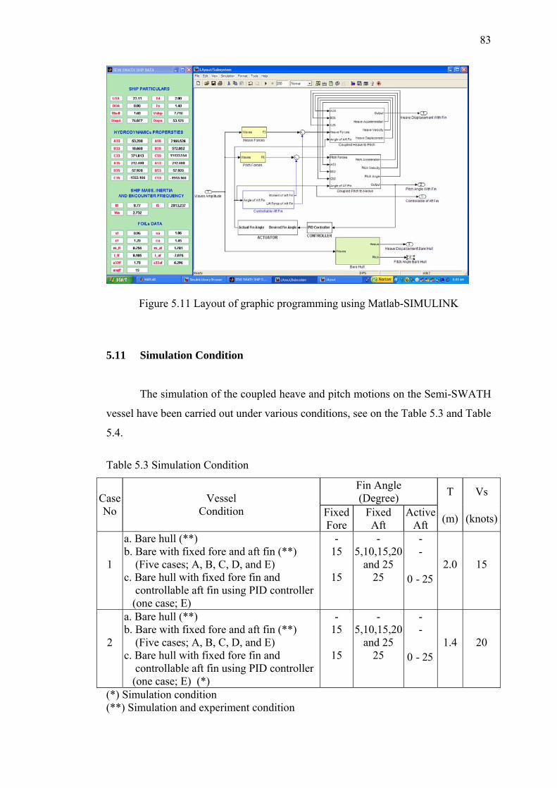
83
Figure 5.11 Layout of graphic programming using Matlab-SIMULINK
5.11 Simulation Condition
The simulation of the coupled heave and pitch motions on the Semi-SWATH
vessel have been carried out under various conditions, see on the Table 5.3 and Table
5.4.
Table 5.3 Simulation Condition
Fin Angle (Degree) T Vs Case
No Vessel
Condition Fixed Fore
Fixed Aft
Active Aft (m) (knots)
1
a. Bare hull (**) b. Bare with fixed fore and aft fin (**) (Five cases; A, B, C, D, and E) c. Bare hull with fixed fore fin and controllable aft fin using PID controller (one case; E)
- 15
15
- 5,10,15,20
and 25 25
- -
0 - 25
2.0
15
2
a. Bare hull (**) b. Bare with fixed fore and aft fin (**) (Five cases; A, B, C, D, and E) c. Bare hull with fixed fore fin and controllable aft fin using PID controller (one case; E) (*)
- 15
15
- 5,10,15,20
and 25 25
- -
0 - 25
1.4
20
(*) Simulation condition (**) Simulation and experiment condition
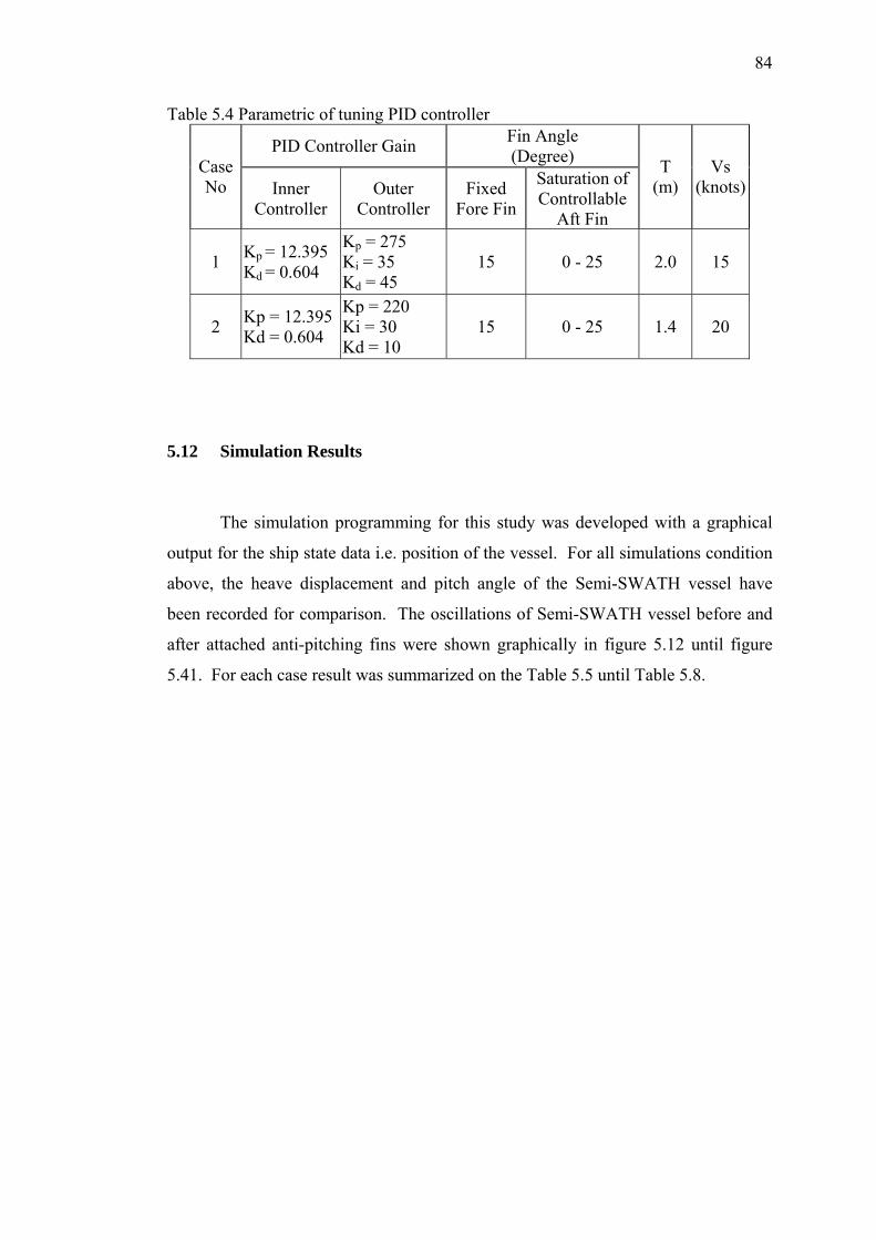
84
Table 5.4 Parametric of tuning PID controller
PID Controller Gain Fin Angle (Degree) Case
No Inner Controller
Outer Controller
Fixed Fore Fin
Saturation of Controllable
Aft Fin
T (m)
Vs (knots)
1 Kp = 12.395 Kd = 0.604
Kp = 275 Ki = 35 Kd = 45
15 0 - 25 2.0 15
2 Kp = 12.395 Kd = 0.604
Kp = 220 Ki = 30 Kd = 10
15 0 - 25 1.4 20
5.12 Simulation Results
The simulation programming for this study was developed with a graphical
output for the ship state data i.e. position of the vessel. For all simulations condition
above, the heave displacement and pitch angle of the Semi-SWATH vessel have
been recorded for comparison. The oscillations of Semi-SWATH vessel before and
after attached anti-pitching fins were shown graphically in figure 5.12 until figure
5.41. For each case result was summarized on the Table 5.5 until Table 5.8.
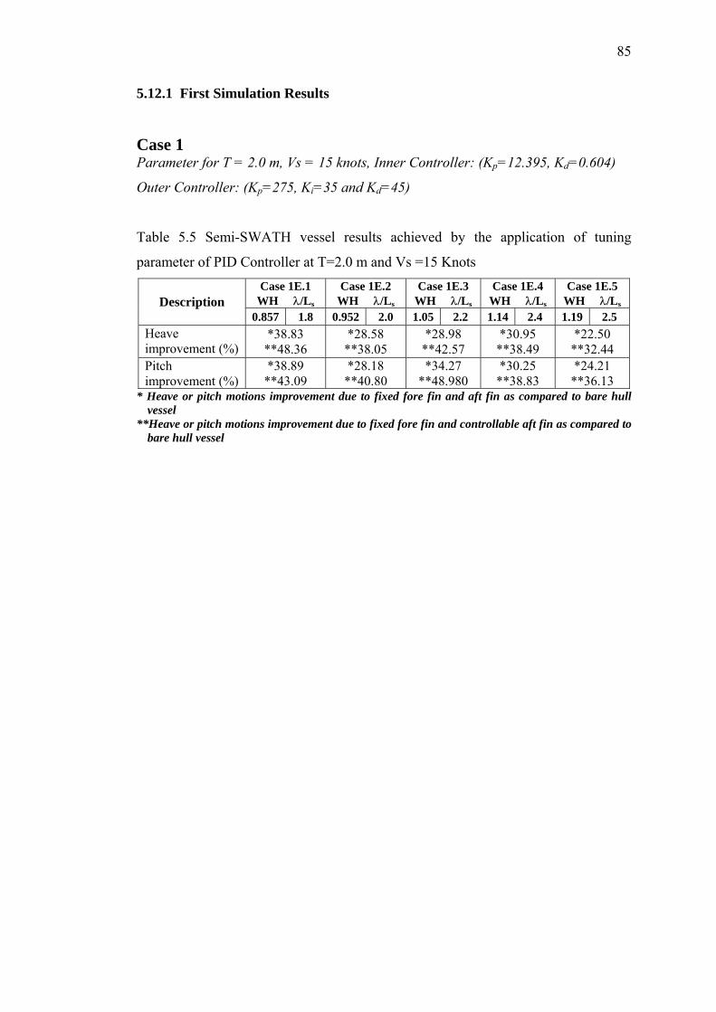
85
5.12.1 First Simulation Results
Case 1 Parameter for T = 2.0 m, Vs = 15 knots, Inner Controller: (Kp=12.395, Kd=0.604)
Outer Controller: (Kp=275, Ki=35 and Kd=45)
Table 5.5 Semi-SWATH vessel results achieved by the application of tuning
parameter of PID Controller at T=2.0 m and Vs =15 Knots Case 1E.1
WH λ/Ls Case 1E.2
WH λ/Ls Case 1E.3
WH λ/Ls Case 1E.4
WH λ/Ls Case 1E.5
WH λ/Ls Description 0.857 1.8 0.952 2.0 1.05 2.2 1.14 2.4 1.19 2.5
Heave improvement (%)
*38.83 **48.36
*28.58 **38.05
*28.98 **42.57
*30.95 **38.49
*22.50 **32.44
Pitch improvement (%)
*38.89 **43.09
*28.18 **40.80
*34.27 **48.980
*30.25 **38.83
*24.21 **36.13
* Heave or pitch motions improvement due to fixed fore fin and aft fin as compared to bare hull vessel
**Heave or pitch motions improvement due to fixed fore fin and controllable aft fin as compared to bare hull vessel
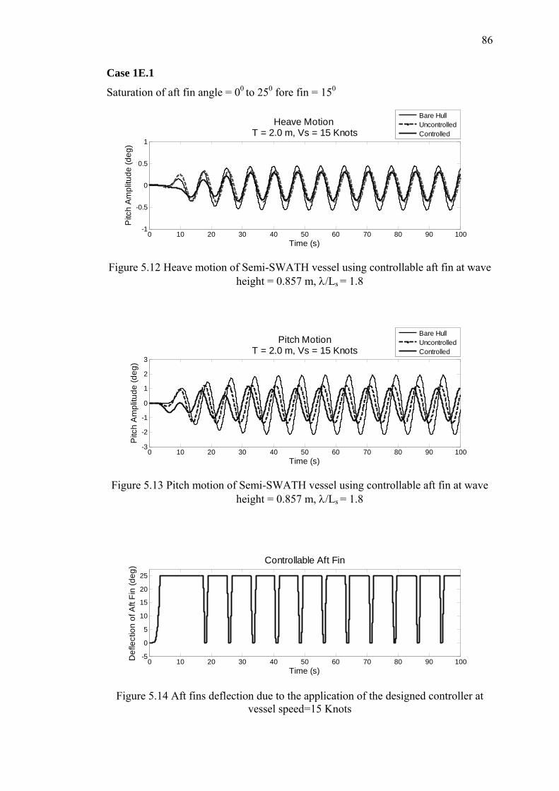
86
Case 1E.1
Saturation of aft fin angle = 00 to 250 fore fin = 150
Bare HullUncontrolledControlled
0 10 20 30 40 50 60 70 80 90 100-1
-0.5
0
0.5
1
Time (s)
Pitc
h A
mpl
itude
(deg
)Heave Motion
T = 2.0 m, Vs = 15 Knots
Figure 5.12 Heave motion of Semi-SWATH vessel using controllable aft fin at wave
height = 0.857 m, λ/Ls = 1.8
0 10 20 30 40 50 60 70 80 90 100-3
-2
-1
0
1
2
3
Time (s)
Pitc
h A
mpl
itude
(deg
)
Pitch MotionT = 2.0 m, Vs = 15 Knots
Bare HullUncontrolledControlled
Figure 5.13 Pitch motion of Semi-SWATH vessel using controllable aft fin at wave
height = 0.857 m, λ/Ls = 1.8
0 10 20 30 40 50 60 70 80 90 100-5
0
5
10
15
20
25
Time (s)
Def
lect
ion
of A
ft Fi
n (d
eg) Controllable Aft Fin
Figure 5.14 Aft fins deflection due to the application of the designed controller at
vessel speed=15 Knots
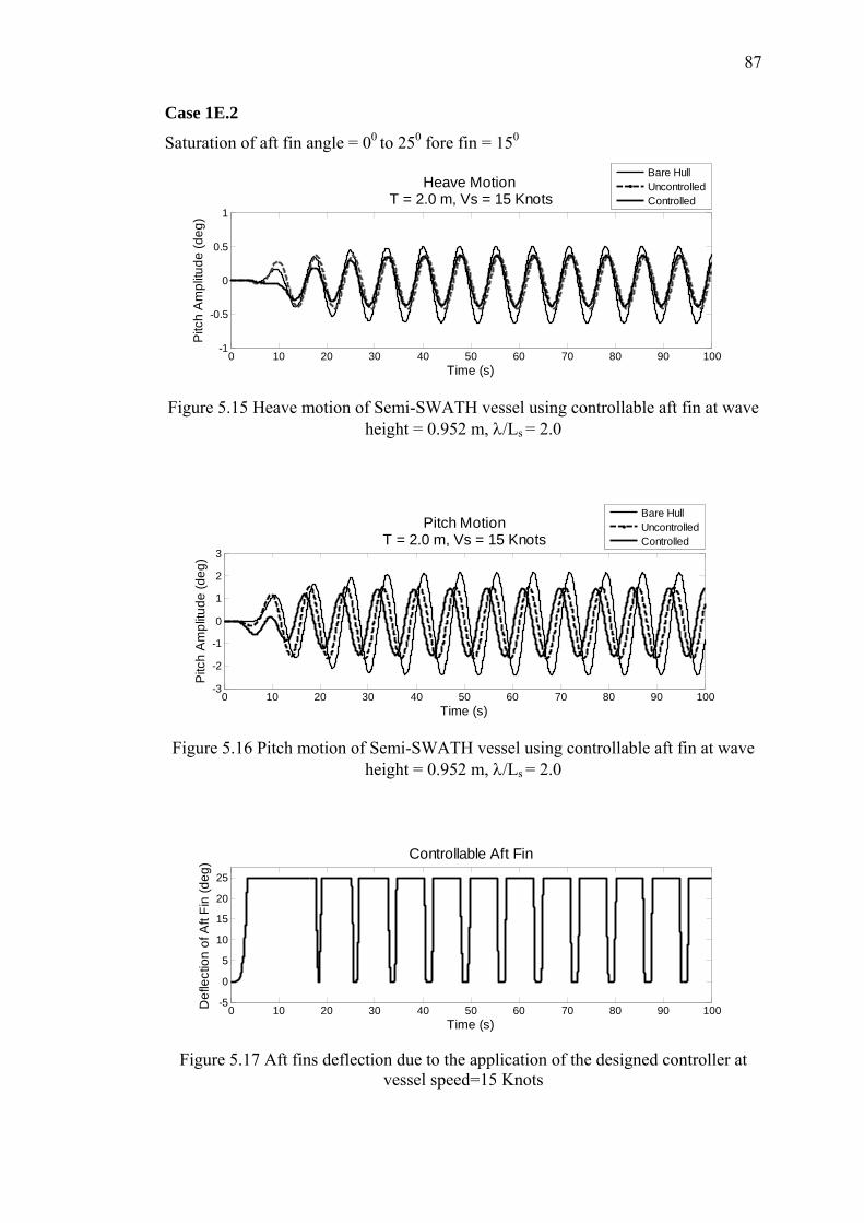
87
Case 1E.2
Saturation of aft fin angle = 00 to 250 fore fin = 150 Bare HullUncontrolledControlled
0 10 20 30 40 50 60 70 80 90 100-1
-0.5
0
0.5
1
Time (s)
Pitc
h A
mpl
itude
(deg
)Heave Motion
T = 2.0 m, Vs = 15 Knots
Figure 5.15 Heave motion of Semi-SWATH vessel using controllable aft fin at wave
height = 0.952 m, λ/Ls = 2.0
Bare HullUncontrolledControlled
0 10 20 30 40 50 60 70 80 90 100-3
-2
-1
0
1
2
3
Time (s)
Pitc
h A
mpl
itude
(deg
)
Pitch MotionT = 2.0 m, Vs = 15 Knots
Figure 5.16 Pitch motion of Semi-SWATH vessel using controllable aft fin at wave
height = 0.952 m, λ/Ls = 2.0
0 10 20 30 40 50 60 70 80 90 100-5
0
5
10
15
20
25
Time (s)
Def
lect
ion
of A
ft Fi
n (d
eg) Controllable Aft Fin
Figure 5.17 Aft fins deflection due to the application of the designed controller at vessel speed=15 Knots
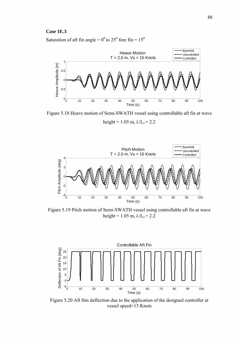
88
Case 1E.3
Saturation of aft fin angle = 00 to 250 fore fin = 150
0 10 20 30 40 50 60 70 80 90 100-1
-0.5
0
0.5
1
Time (s)
Hea
ve A
mpl
itude
(m)
Heave Motion T = 2.0 m, Vs = 15 Knots
BareHullUncontrolledControlled
Figure 5.18 Heave motion of Semi-SWATH vessel using controllable aft fin at wave
height = 1.05 m, λ/Ls = 2.2
BareHullUncontrolledControlled
0 10 20 30 40 50 60 70 80 90 100-4
-2
0
2
4
Time (s)
Pitc
h A
mpl
itude
(deg
)
Pitch MotionT = 2.0 m, Vs = 15 Knots
Figure 5.19 Pitch motion of Semi-SWATH vessel using controllable aft fin at wave
height = 1.05 m, λ/Ls = 2.2
0 10 20 30 40 50 60 70 80 90 100-5
0
5
10
15
20
25
Time (s)
Def
lect
ion
of A
ft Fi
n (d
eg) Controllable Aft Fin
Figure 5.20 Aft fins deflection due to the application of the designed controller at
vessel speed=15 Knots
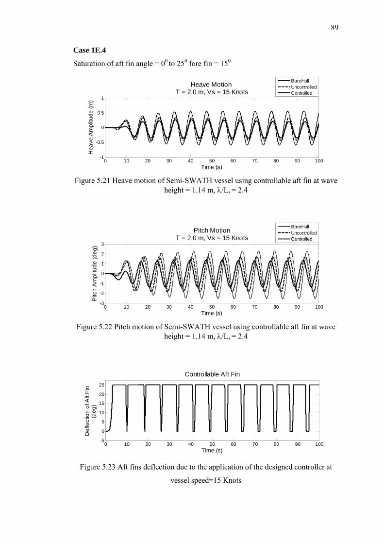
89
Case 1E.4
Saturation of aft fin angle = 00 to 250 fore fin = 150
0 10 20 30 40 50 60 70 80 90 100-1
-0.5
0
0.5
1
Time (s)
Hea
ve A
mpl
itude
(m)
Heave Motion T = 2.0 m, Vs = 15 Knots
BareHullUncontrolledControlled
Figure 5.21 Heave motion of Semi-SWATH vessel using controllable aft fin at wave
height = 1.14 m, λ/Ls = 2.4
BareHullUncontrolledControlled
0 10 20 30 40 50 60 70 80 90 100-3
-2
-1
0
1
2
3
Time (s)
Pitc
h A
mpl
itude
(deg
)
Pitch MotionT = 2.0 m, Vs = 15 Knots
Figure 5.22 Pitch motion of Semi-SWATH vessel using controllable aft fin at wave
height = 1.14 m, λ/Ls = 2.4
0 10 20 30 40 50 60 70 80 90 100-5
0
5
10
15
20
25
Time (s)
Def
lect
ion
of A
ft Fi
n
(deg
)
Controllable Aft Fin
Figure 5.23 Aft fins deflection due to the application of the designed controller at
vessel speed=15 Knots
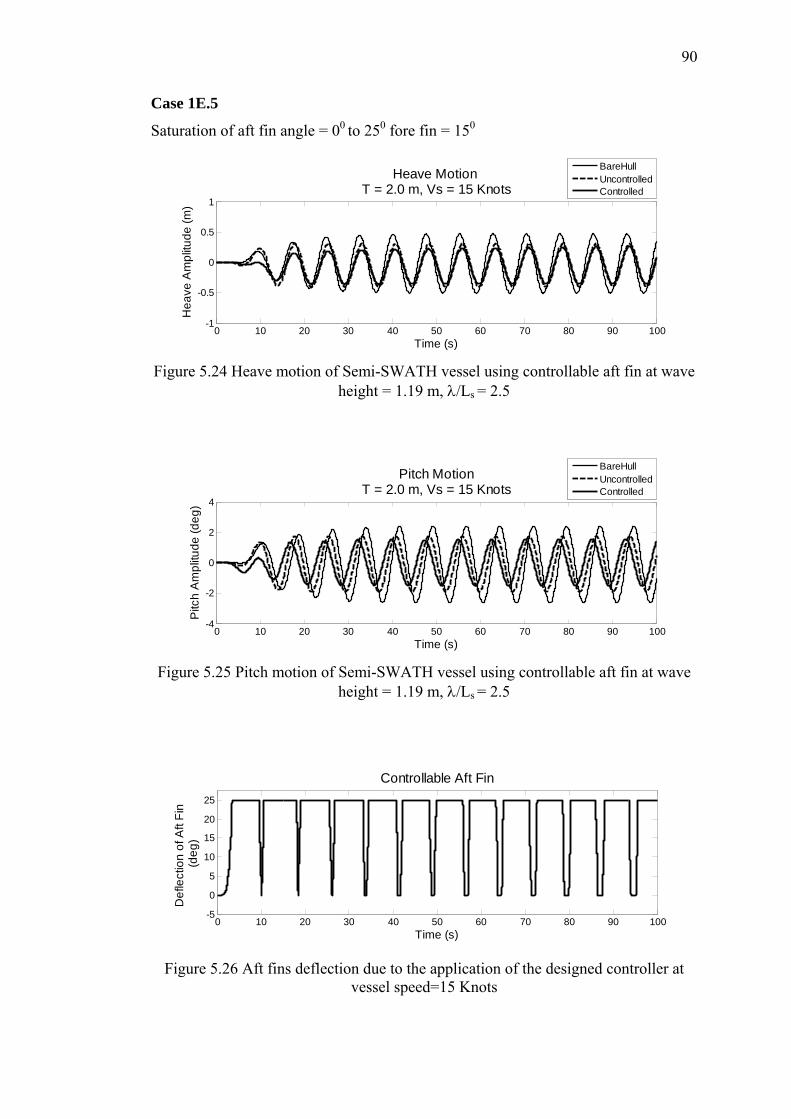
90
Case 1E.5
Saturation of aft fin angle = 00 to 250 fore fin = 150
0 10 20 30 40 50 60 70 80 90 100-1
-0.5
0
0.5
1
Time (s)
Hea
ve A
mpl
itude
(m)
Heave Motion T = 2.0 m, Vs = 15 Knots
BareHullUncontrolledControlled
Figure 5.24 Heave motion of Semi-SWATH vessel using controllable aft fin at wave
height = 1.19 m, λ/Ls = 2.5
BareHullUncontrolledControlled
0 10 20 30 40 50 60 70 80 90 100-4
-2
0
2
4
Time (s)
Pitc
h A
mpl
itude
(deg
)
Pitch MotionT = 2.0 m, Vs = 15 Knots
Figure 5.25 Pitch motion of Semi-SWATH vessel using controllable aft fin at wave
height = 1.19 m, λ/Ls = 2.5
0 10 20 30 40 50 60 70 80 90 100-5
0
5
10
15
20
25
Time (s)
Def
lect
ion
of A
ft Fi
n (d
eg)
Controllable Aft Fin
Figure 5.26 Aft fins deflection due to the application of the designed controller at
vessel speed=15 Knots
91
5.12.2 Second Simulation Results
Case 2 Parameter for T =1.4 m, Vs = 20 knots, Inner Controller: (Kp=12.395, Kd=0.604)
Outer Controller: (Kp=275, Ki=35 and Kd=45)
Table 5.6 Semi-SWATH vessel results achieved by the application of tuning
parameter of PID Controller at T=1.4 m and Vs =20 Knots Case 2E.1
WH λ/Ls Case 2E.2
WH λ/Ls Case 2E.3
WH λ/Ls Case 2E.4
WH λ/Ls Case 2E.5
WH λ/Ls Description 0.4285 1 0.476 1.2 0.525 1.4 0.57 1.6 0.595 1.8
Heave improvement (%) 15.393 12.211 13.663 26.775 17.882
Pitch improvement (%) 12.473 9.628 11.264 17.152 25.771
In Table 5.6, shown the improvement of heave and pitch motions due to application
of PID Controller on the controllable aft fins (saturation of aft fin angle = 00 – 250) as
compared to the fixed fore and aft fins (fore fin = 150 and aft fin = 250)
92
Case 2E.1
Saturation of aft fin angle = 00 to 250 fore fin = 150
0 10 20 30 40 50 60 70 80 90 100-0.05
0
0.05
0.1
0.15
Time (s)
Hea
ve A
mpl
itude
(m)
Heave Motion T = 2.0 m, Vs = 15 Knots
UncontrolledControlled
Figure 5.27 Heave motion on the Semi-SWATH vessel at wave height = 0.476 m,
λ/Ls = 1
UncontrolledControlled
0 10 20 30 40 50 60 70 80 90 100-1
-0.5
0
0.5
1
1.5
Time (s)
Pitc
h A
mpl
itude
(deg
)
Pitch MotionT = 1.4 m, Vs = 20 Knots
Figure 5.28 Pitch motion on the Semi-SWATH vessel at wave height = 0.476 m, λ/Ls
= 1
0 10 20 30 40 50 60 70 80 90 100-5
0
5
10
15
20
25
Time (s)
Def
lect
ion
of A
ft Fi
n
(d
eg)
Controllable Aft Fin
Figure 5.29 Aft fins deflection due to the application of the designed controller at
vessel speed=15 Knots
93
Case 2E.2
Saturation of aft fin angle = 00 to 250 fore fin = 150
0 10 20 30 40 50 60 70 80 90 100-0.2
-0.1
0
0.1
0.2
0.3
Time (s)
Hea
ve A
mpl
itude
(m)
Heave Motion T = 2.0 m, Vs = 15 Knots
UncontrolledControlled
Figure 5.30 Heave motion on the Semi-SWATH vessel at wave height = 0.571 m,
λ/Ls = 1.2
UncontrolledControlled
0 10 20 30 40 50 60 70 80 90 100-2
-1
0
1
2
3
4
Time (s)
Pitc
h A
mpl
itude
(deg
)
Pitch MotionT = 1.4 m, Vs = 20 Knots
Figure 5.31 Pitch motion on the Semi-SWATH vessel at wave height = 0.571 m, λ/Ls
= 1.2
0 10 20 30 40 50 60 70 80 90 100-5
0
5
10
15
20
25
Time (s)
Def
lect
ion
of A
ft Fi
n
(d
eg)
Controllable Aft Fin
Figure 5.32 Aft fins deflection due to the application of the designed controller at vessel speed=15 Knots
94
Case 2E.3
Saturation of aft fin angle = 00 to 250 fore fin = 150
0 10 20 30 40 50 60 70 80 90 100-0.2
-0.1
0
0.1
0.2
0.3
Time (s)
Hea
ve A
mpl
itude
(m)
Heave Motion T = 2.0 m, Vs = 15 Knots
UncontrolledControlled
Figure 5.33 Heave motion on the Semi-SWATH vessel at wave height = 0.666 m,
λ/Ls = 1.4
UncontrolledControlled
0 10 20 30 40 50 60 70 80 90 100-2
-1
0
1
2
3
4
Time (s)
Pitc
h A
mpl
itude
(deg
)
Pitch MotionT = 1.4 m, Vs = 20 Knots
Figure 5.34 Pitch motion on the Semi-SWATH vessel at wave height = 0.666 m, λ/Ls
= 1.4
0 10 20 30 40 50 60 70 80 90 100-5
0
5
10
15
20
25
Time (s)
Def
lect
ion
of A
ft Fi
n (d
eg)
Controllable Aft Fin
Figure 5.35 Aft fins deflection due to the application of the designed controller at
vessel speed=15 Knots
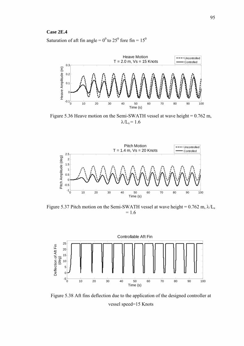
95
Case 2E.4
Saturation of aft fin angle = 00 to 250 fore fin = 150
0 10 20 30 40 50 60 70 80 90 100-0.1
0
0.1
0.2
0.3
Time (s)
Hea
ve A
mpl
itude
(m)
Heave Motion T = 2.0 m, Vs = 15 Knots
UncontrolledControlled
Figure 5.36 Heave motion on the Semi-SWATH vessel at wave height = 0.762 m,
λ/Ls = 1.6
UncontrolledControlled
0 10 20 30 40 50 60 70 80 90 100-1
-0.5
0
0.5
1
1.5
2
2.5
Time (s)
Pitc
h A
mpl
itude
(deg
)
Pitch MotionT = 1.4 m, Vs = 20 Knots
Figure 5.37 Pitch motion on the Semi-SWATH vessel at wave height = 0.762 m, λ/Ls
= 1.6
0 10 20 30 40 50 60 70 80 90 100-5
0
5
10
15
20
25
Time (s)
Def
lect
ion
of A
ft Fi
n
(deg
)
Controllable Aft Fin
Figure 5.38 Aft fins deflection due to the application of the designed controller at
vessel speed=15 Knots
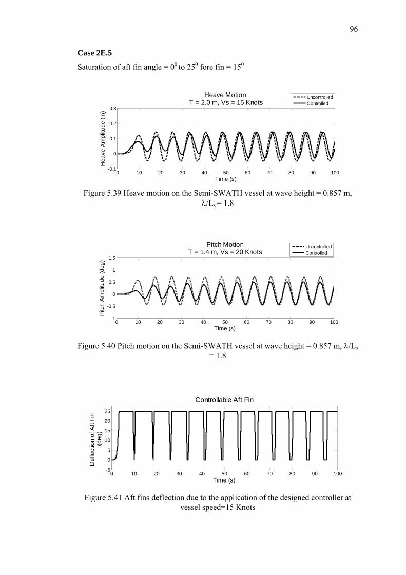
96
Case 2E.5
Saturation of aft fin angle = 00 to 250 fore fin = 150
0 10 20 30 40 50 60 70 80 90 100-0.1
0
0.1
0.2
0.3
Time (s)
Hea
ve A
mpl
itude
(m)
Heave Motion T = 2.0 m, Vs = 15 Knots
UncontrolledControlled
Figure 5.39 Heave motion on the Semi-SWATH vessel at wave height = 0.857 m,
λ/Ls = 1.8
UncontrolledControlled
0 10 20 30 40 50 60 70 80 90 100-1
-0.5
0
0.5
1
1.5
Time (s)
Pitc
h A
mpl
itude
(deg
)
Pitch MotionT = 1.4 m, Vs = 20 Knots
Figure 5.40 Pitch motion on the Semi-SWATH vessel at wave height = 0.857 m, λ/Ls
= 1.8
0 10 20 30 40 50 60 70 80 90 100-5
0
5
10
15
20
25
Time (s)
Def
lect
ion
of A
ft Fi
n (d
eg)
Controllable Aft Fin
Figure 5.41 Aft fins deflection due to the application of the designed controller at
vessel speed=15 Knots
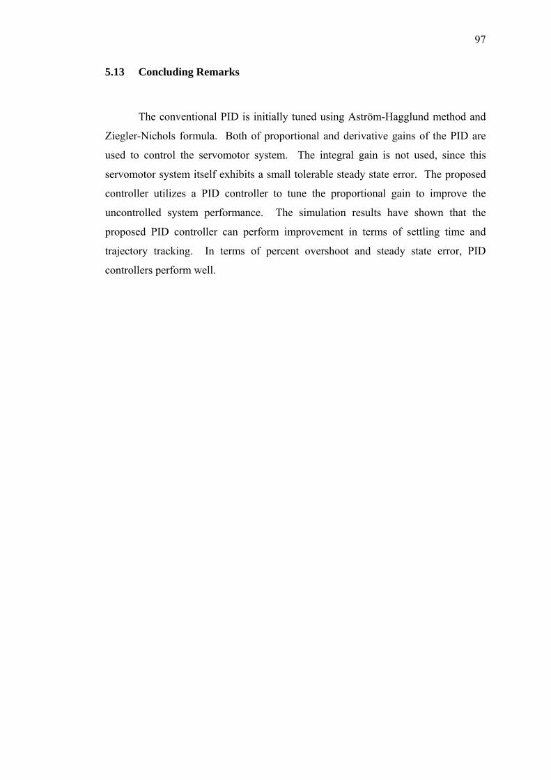
97
5.13 Concluding Remarks
The conventional PID is initially tuned using Aström-Hagglund method and
Ziegler-Nichols formula. Both of proportional and derivative gains of the PID are
used to control the servomotor system. The integral gain is not used, since this
servomotor system itself exhibits a small tolerable steady state error. The proposed
controller utilizes a PID controller to tune the proportional gain to improve the
uncontrolled system performance. The simulation results have shown that the
proposed PID controller can perform improvement in terms of settling time and
trajectory tracking. In terms of percent overshoot and steady state error, PID
controllers perform well.
CHAPTER 6
PROCEDURE OF SEAKEEPING TEST
6.1 General
Generally, the seakeeping model tests in a towing tank are the most
preferable option to validate the trusted results from the simulation programs. In
addition, the quality of the tests is determined by the model scale and by the number
of oscillations that the model experience in the test length (Lloyd, 1989).
Consequently, it was needed a better understanding of all involved parameters of this
test as well.
Accordingly, in this chapter is emphasized to describe the seakeeping model
test properties such as objective of experiment, the model ship, test facility, and the
procedures employed in designing the experiment.
6.2 Objective of The Experiments
Experimental seakeeping test was carried out on the Semi-SWATH model in
regular head seas condition. The towed Semi-SWATH model was tested both with
and without fin stabilizers. The heave and pitch motion responses of the model as
the output recorded data during experiments.
99
Therefore, the objective of this experiment is to validate the simulation
program results in case of the vertical motion (heave and pitch motions)
characteristics of Semi-SWATH vessel. Then, the motion responses of heave and
pitch including the significant status of the behavior of the vessel will be evaluated.
Next the author present to the situation of these experiments on the RAOs of the
Semi-SWATH vessel with and without fin stabilizers. Finally, the responses of the
model to the same speed and waves will be compared correspondingly.
6.3 Model Test Preparation
The experiment was conducted by using the scaled model of Semi-SWATH
with the scale factor of 1:10 the particulars of model will be described in sub-chapter
6.3.1. The static preparation of the model consists of establishing its weight
distribution to corresponding to the full scale ship. In other words, the ratio of the
masses of homologous sections of the full-scale vessel and the model should be the
cube of the scale ratio. From the Froude’s laws, the scaling relationships governed
only consider inertia and gravity forces. Although Froude's law does not satisfy the
scaling laws concerning fluid compressibility, viscosity, surface tension, and so on,
the effects of these factors are insignificant as far as seakeeping characteristics are
concerned.
In order to have the ship weight distribution correspond in model scale,
generally the following conditions must be satisfied (for the detail see Table 6.1):
• Total weight or displacement.
• Net longitudinal position of the center of gravity for trim purposes.
• Radius of gyration
For model to have weight distribution in model scale, the model should be
ballasted by arranging weights correctly to scale so the model at draught
corresponding to full scale ship. The center of gravity of the model should be
determined in order to corresponding to ships center of gravity. The correct height
position of the center of mass of model is achieved by a heeling test of the oscillation
table.
100
After the model ready in the needed condition researcher will proceed to next
process with make the experiment set-up. In this step, researcher must make sure all
equipment involve in the experiment are in good condition to make sure the result of
the experiment is available to used.
6.3.1 Model Test Particulars
The semi-SWATH model was designed and decided to make the models
2.31m long, giving a scale of 1:10. It had buoyancy distribution to the Semi-
SWATH hull at the scaled nominal displacements. This guaranteed the same scaled
nominal wetted lengths and draughts in the variable loadings of the model test
conditions. For the detail of model test particular was summarized in the Table 6.1.
In addition, the variable draughts of the model test were conducted for two draught
operations i.e. a light draught by 14 cm (corresponding to 53.176 kg) and a full-load
draught by 20 cm (corresponding to 76.877 kg). This arrangement was set up using
ballasted weight.
In this experiment, the seakeeping test will be conducted both to the bare hull
model and after attached fin stabilizers. The principle dimensions corresponding to
the fin stabilizers are shown in Table 6.2. Furthermore, the completed Semi-
SWATH model configurations after installed of fin stabilizers were shown
respectively in figure 6.1 and 6.2.
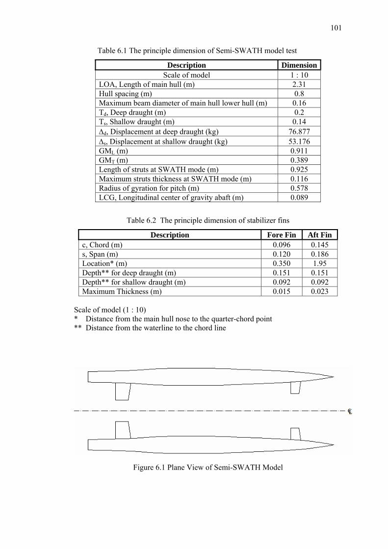
101
Table 6.1 The principle dimension of Semi-SWATH model test
Description Dimension Scale of model 1 : 10
LOA, Length of main hull (m) 2.31 Hull spacing (m) 0.8 Maximum beam diameter of main hull lower hull (m) 0.16 Td, Deep draught (m) 0.2 Ts, Shallow draught (m) 0.14 ∆d, Displacement at deep draught (kg) 76.877 ∆s, Displacement at shallow draught (kg) 53.176 GML (m) 0.911 GMT (m) 0.389 Length of struts at SWATH mode (m) 0.925 Maximum struts thickness at SWATH mode (m) 0.116 Radius of gyration for pitch (m) 0.578 LCG, Longitudinal center of gravity abaft (m) 0.089
Table 6.2 The principle dimension of stabilizer fins
Description Fore Fin Aft Fin c, Chord (m) 0.096 0.145 s, Span (m) 0.120 0.186 Location* (m) 0.350 1.95 Depth** for deep draught (m) 0.151 0.151 Depth** for shallow draught (m) 0.092 0.092 Maximum Thickness (m) 0.015 0.023
Scale of model (1 : 10) * Distance from the main hull nose to the quarter-chord point ** Distance from the waterline to the chord line
Figure 6.1 Plane View of Semi-SWATH Model
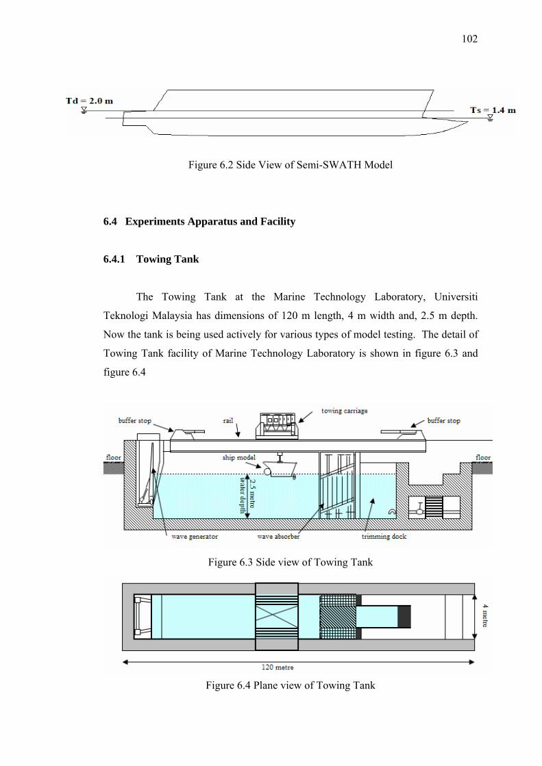
102
Figure 6.2 Side View of Semi-SWATH Model
6.4 Experiments Apparatus and Facility
6.4.1 Towing Tank
The Towing Tank at the Marine Technology Laboratory, Universiti
Teknologi Malaysia has dimensions of 120 m length, 4 m width and, 2.5 m depth.
Now the tank is being used actively for various types of model testing. The detail of
Towing Tank facility of Marine Technology Laboratory is shown in figure 6.3 and
figure 6.4
Figure 6.3 Side view of Towing Tank
Figure 6.4 Plane view of Towing Tank
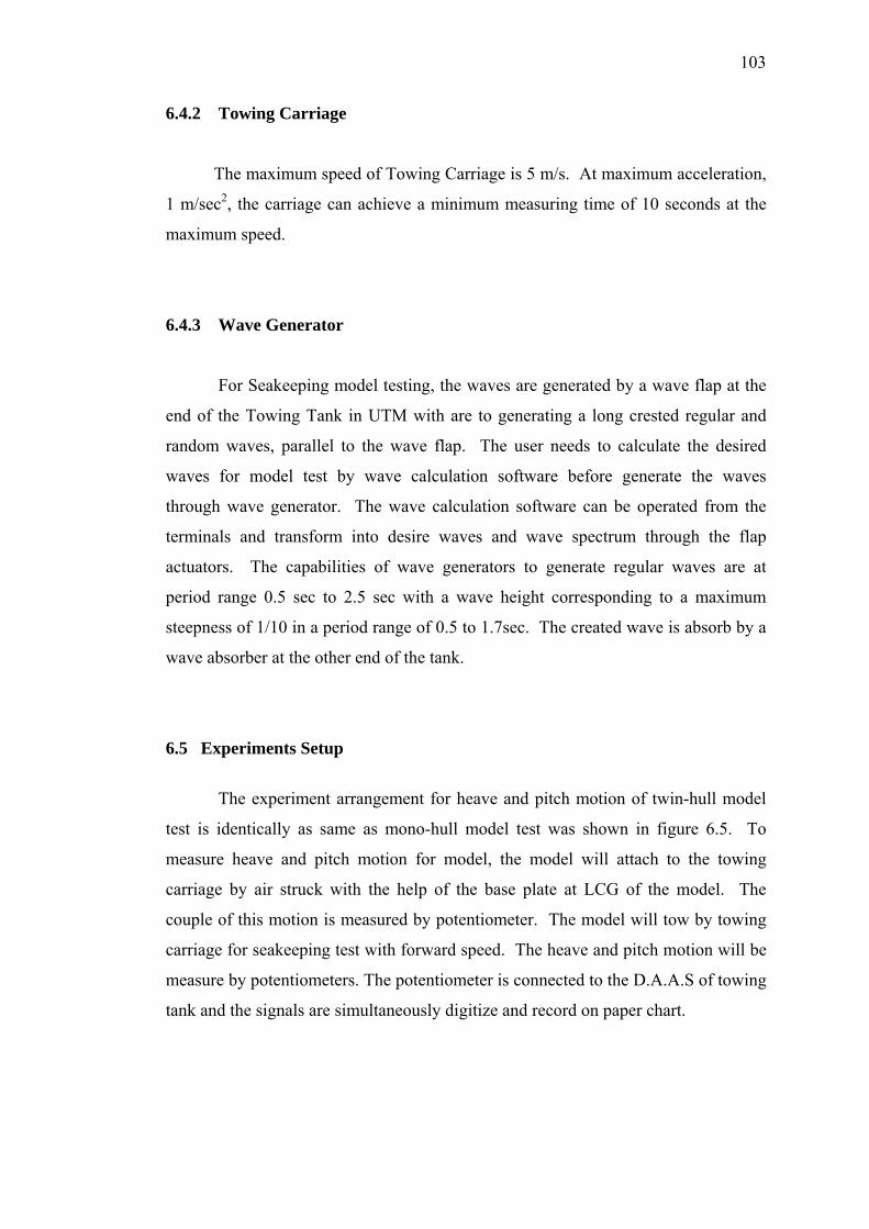
103
6.4.2 Towing Carriage
The maximum speed of Towing Carriage is 5 m/s. At maximum acceleration,
1 m/sec2, the carriage can achieve a minimum measuring time of 10 seconds at the
maximum speed.
6.4.3 Wave Generator
For Seakeeping model testing, the waves are generated by a wave flap at the
end of the Towing Tank in UTM with are to generating a long crested regular and
random waves, parallel to the wave flap. The user needs to calculate the desired
waves for model test by wave calculation software before generate the waves
through wave generator. The wave calculation software can be operated from the
terminals and transform into desire waves and wave spectrum through the flap
actuators. The capabilities of wave generators to generate regular waves are at
period range 0.5 sec to 2.5 sec with a wave height corresponding to a maximum
steepness of 1/10 in a period range of 0.5 to 1.7sec. The created wave is absorb by a
wave absorber at the other end of the tank.
6.5 Experiments Setup
The experiment arrangement for heave and pitch motion of twin-hull model
test is identically as same as mono-hull model test was shown in figure 6.5. To
measure heave and pitch motion for model, the model will attach to the towing
carriage by air struck with the help of the base plate at LCG of the model. The
couple of this motion is measured by potentiometer. The model will tow by towing
carriage for seakeeping test with forward speed. The heave and pitch motion will be
measure by potentiometers. The potentiometer is connected to the D.A.A.S of towing
tank and the signals are simultaneously digitize and record on paper chart.
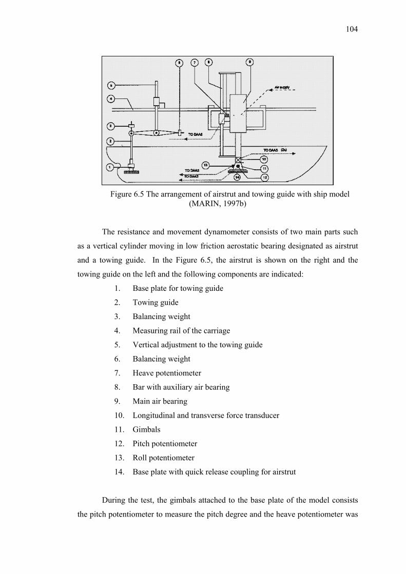
104
Figure 6.5 The arrangement of airstrut and towing guide with ship model (MARIN, 1997b)
The resistance and movement dynamometer consists of two main parts such
as a vertical cylinder moving in low friction aerostatic bearing designated as airstrut
and a towing guide. In the Figure 6.5, the airstrut is shown on the right and the
towing guide on the left and the following components are indicated:
1. Base plate for towing guide
2. Towing guide
3. Balancing weight
4. Measuring rail of the carriage
5. Vertical adjustment to the towing guide
6. Balancing weight
7. Heave potentiometer
8. Bar with auxiliary air bearing
9. Main air bearing
10. Longitudinal and transverse force transducer
11. Gimbals
12. Pitch potentiometer
13. Roll potentiometer
14. Base plate with quick release coupling for airstrut
During the test, the gimbals attached to the base plate of the model consists
the pitch potentiometer to measure the pitch degree and the heave potentiometer was
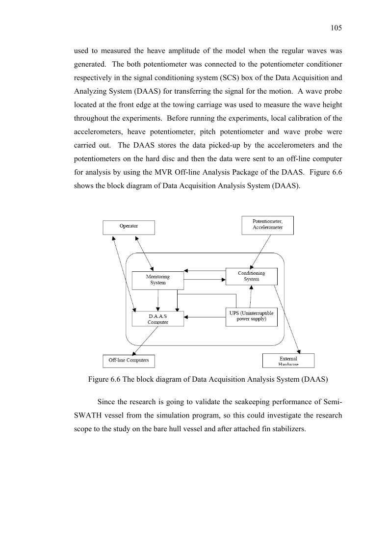
105
used to measured the heave amplitude of the model when the regular waves was
generated. The both potentiometer was connected to the potentiometer conditioner
respectively in the signal conditioning system (SCS) box of the Data Acquisition and
Analyzing System (DAAS) for transferring the signal for the motion. A wave probe
located at the front edge at the towing carriage was used to measure the wave height
throughout the experiments. Before running the experiments, local calibration of the
accelerometers, heave potentiometer, pitch potentiometer and wave probe were
carried out. The DAAS stores the data picked-up by the accelerometers and the
potentiometers on the hard disc and then the data were sent to an off-line computer
for analysis by using the MVR Off-line Analysis Package of the DAAS. Figure 6.6
shows the block diagram of Data Acquisition Analysis System (DAAS).
Figure 6.6 The block diagram of Data Acquisition Analysis System (DAAS)
Since the research is going to validate the seakeeping performance of Semi-
SWATH vessel from the simulation program, so this could investigate the research
scope to the study on the bare hull vessel and after attached fin stabilizers.
106
6.6 Experiment Condition
Calculation conditions for the Semi-SWATH model Seakeeping prediction
are base on the requirement given as follow:
• Motion amplitudes for heave and pitch in head sea with forward speed of 20
knots. Froude Number, Fn = 0.684
• Motion amplitudes for heave and pitch in head sea with forward speed of 20
knots Froude Number, Fn = 0.512
The ship motion prediction in waves was carried out at the following
environmental condition:
• A range of regular wave lengths: 0.5 ≤ λ/L ≤ 2.5
• Steepness of the incident wave: H/λ = 1/50
For measuring the heave and pitch motion, the model is arranged to head sea
condition with regular waves of various periods. The model is tested at two different
Froude Number such as 0.684 and 0.512 with two variable draughts.
6.7 Description of Data Test Analysis
Since in the regular wave analysis all data should be nominally periodic in
time, the basic procedure was to perform a harmonic analysis on all data channel for
extracting the fundamental harmonics and for determining the transfer functions
between the wave input and motion response output.
The heave displacement, pitch degree, accelerations and wave amplitude
signals in time-domain was picked up by the heave potentiometer, pitch
potentiometer and accelerometers were recorded. Using the MVR Off-line Analysis
Package of the DAAS then processed the raw signals. By using the MVR software,
the raw signals picked up were processed by the option named plotsim subjected in
Output to plot the signals of all the measurements in time-domain. The option To
107
ASCII subjected in Tools also in the MVR software was used to transfer the data in
type of Tab.
In the data test analysis, the wave input and motion response output of heave
and pitch will be analyzed using Response Amplitude Operators (RAOs). This term
is to describe and determine the significant heave amplitude and determine
significant pitch amplitude divide by wave amplitude. Presented quantities are made
non-dimensional, as follows: heave and pitch divided by wave amplitude and
Standard International Metric Units were used throughout. The formulation of the
RAOs is presented in equation 6.1.
a
a
u motion amplitude = ξ wave ampitude
(6.1)
Where; au can be defined as heave amplitude (m) or pitch amplitude (degree).
Finally, the heave and pitch responses per unit wave height are similarly
plotted for every cycle of seakeeping tests. Included in the diagrams are curves
showing the ratio of the heave and pitch motions of the Semi-SWATH model with
fins and without fins. The advanced analysis of the motion responses the RAO
results are plotted against to the wavelength and ship length ratio (Ship
λL
).
6.8 Concluding Remarks
The seakeeping test of Semi-SWATH model is carried out in Towing Tank of
Marine Technology Laboratory and restricted only to regular head condition. In this
experiments, the range ratio of wavelengths to the model length (Ship
λL
) is about 0.5-
2.5 with wave height to wavelength ratio at the experiments was 1/25. The measured
data from all channels were digitized at a rate of 25 samples per second on each
channel. Where, the total number of encounter cycles collected on each run was
typically between 5 and 10 times. Then, all data channels are extracted using MVR
software. Finally, the result data analysis of heave and pitch responses will be
108
plotted per unit wave height with fins and without fins as the Response Amplitude
Operators (RAOs) against to the wavelength and ship length ratio (Ship
λL
).
CHAPTER 7
VALIDATION
7.1 General
In this chapter, a comparison between simulation results with the
experimental data provided by the Semi-SWATH model test at Towing Tank of
Marine Technology Laboratory, Universiti Teknologi Malaysia is carried out to
validate the simulation program. Two responses are considered in the comparison;
those are heave and pitch motions.
7.2 Comparison of Experimental and Simulation Results
For comparison, the seakeeping model test of Semi-SWATH with 76.877
tones and 53.176 tones displacement (deep draught and shallow draught respectively)
had been chosen for the investigation of ship motion in waves. There are two cases
specified in the comparison. The summary of the comparison condition is shown in
Table 7.1
For all the conditions both simulations and experiments, the operational
draught is taken as 1.4 m (shallow draught) and 2.0 m (deep draught). Other
conditions had been taken are; wave length to ship length ratio is taken as
/ 1 - 2.5W Lλ = and wave height to length ratio is taking as 25/1/ =WWH λ and
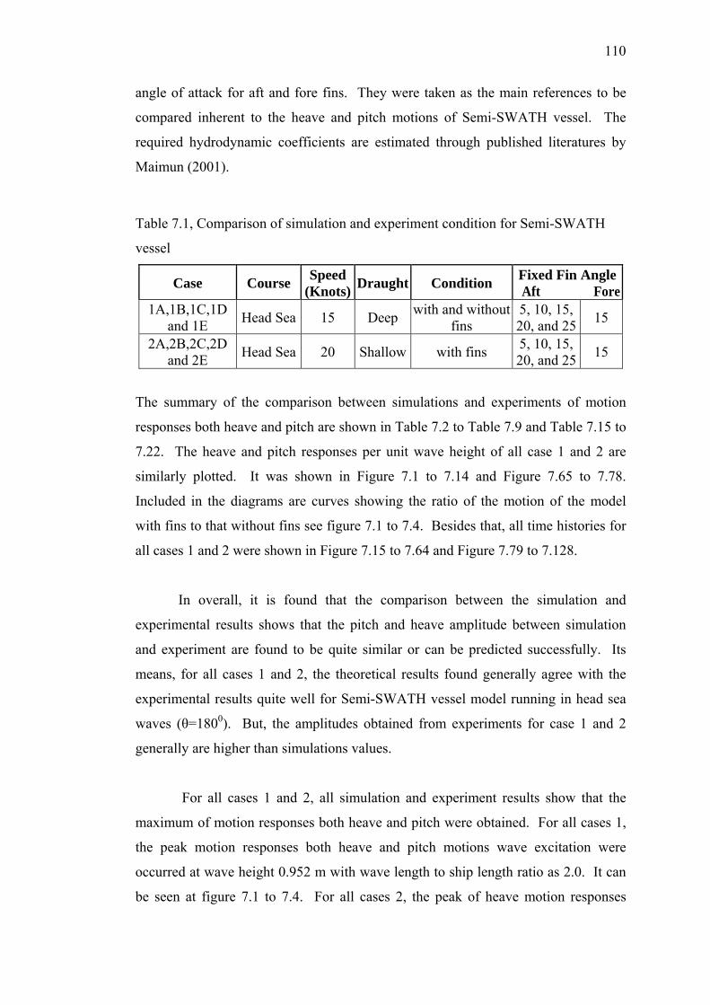
110
angle of attack for aft and fore fins. They were taken as the main references to be
compared inherent to the heave and pitch motions of Semi-SWATH vessel. The
required hydrodynamic coefficients are estimated through published literatures by
Maimun (2001).
Table 7.1, Comparison of simulation and experiment condition for Semi-SWATH
vessel
Case Course Speed (Knots) Draught Condition Fixed Fin Angle
Aft Fore1A,1B,1C,1D
and 1E Head Sea 15 Deep with and without fins
5, 10, 15, 20, and 25 15
2A,2B,2C,2D and 2E Head Sea 20 Shallow with fins 5, 10, 15,
20, and 25 15
The summary of the comparison between simulations and experiments of motion
responses both heave and pitch are shown in Table 7.2 to Table 7.9 and Table 7.15 to
7.22. The heave and pitch responses per unit wave height of all case 1 and 2 are
similarly plotted. It was shown in Figure 7.1 to 7.14 and Figure 7.65 to 7.78.
Included in the diagrams are curves showing the ratio of the motion of the model
with fins to that without fins see figure 7.1 to 7.4. Besides that, all time histories for
all cases 1 and 2 were shown in Figure 7.15 to 7.64 and Figure 7.79 to 7.128.
In overall, it is found that the comparison between the simulation and
experimental results shows that the pitch and heave amplitude between simulation
and experiment are found to be quite similar or can be predicted successfully. Its
means, for all cases 1 and 2, the theoretical results found generally agree with the
experimental results quite well for Semi-SWATH vessel model running in head sea
waves (θ=1800). But, the amplitudes obtained from experiments for case 1 and 2
generally are higher than simulations values.
For all cases 1 and 2, all simulation and experiment results show that the
maximum of motion responses both heave and pitch were obtained. For all cases 1,
the peak motion responses both heave and pitch motions wave excitation were
occurred at wave height 0.952 m with wave length to ship length ratio as 2.0. It can
be seen at figure 7.1 to 7.4. For all cases 2, the peak of heave motion responses
111
generally were occurred at wave height 0.571 m with wave length to ship length ratio
as 1.2. It can be seen at figure 7.65. But, for the peak of pitch motion responses
were occurred at wave height 0.666 m with wave length to ship length ratio as 1.4. It
can be seen at figure 7.66.
The results of the model tests for various angle of fins compared to bare hull
vessel in case 1 showed that the motions of heave and pitch were reduced by a
maximum about;
1. Case 1A
Case 1A.4; heave = 28.522%, pitch = 26.134%
2. Case 1B
Case 1B.1; heave = 34.02%, pitch = 22.00%
3. Case 1C
Case 1C.1; heave = 32.14%, Case 1C.5; pitch = 37.95%
4. Case 1D
Case 1D.5; heave = 39.18%, pitch = 36.52%
5. Case 1E
Case 1E.2; heave = 37.965%, Case 1E.1; pitch = 35.81%
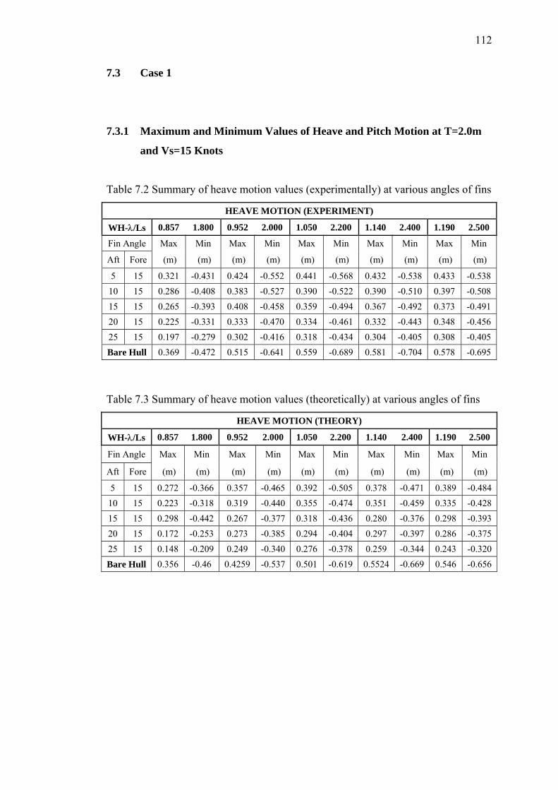
112
7.3 Case 1
7.3.1 Maximum and Minimum Values of Heave and Pitch Motion at T=2.0m
and Vs=15 Knots
Table 7.2 Summary of heave motion values (experimentally) at various angles of fins
HEAVE MOTION (EXPERIMENT)
WH-λ/Ls 0.857 1.800 0.952 2.000 1.050 2.200 1.140 2.400 1.190 2.500
Fin Angle Max Min Max Min Max Min Max Min Max Min
Aft Fore (m) (m) (m) (m) (m) (m) (m) (m) (m) (m)
5 15 0.321 -0.431 0.424 -0.552 0.441 -0.568 0.432 -0.538 0.433 -0.538 10 15 0.286 -0.408 0.383 -0.527 0.390 -0.522 0.390 -0.510 0.397 -0.508 15 15 0.265 -0.393 0.408 -0.458 0.359 -0.494 0.367 -0.492 0.373 -0.491 20 15 0.225 -0.331 0.333 -0.470 0.334 -0.461 0.332 -0.443 0.348 -0.456 25 15 0.197 -0.279 0.302 -0.416 0.318 -0.434 0.304 -0.405 0.308 -0.405 Bare Hull 0.369 -0.472 0.515 -0.641 0.559 -0.689 0.581 -0.704 0.578 -0.695
Table 7.3 Summary of heave motion values (theoretically) at various angles of fins
HEAVE MOTION (THEORY)
WH-λ/Ls 0.857 1.800 0.952 2.000 1.050 2.200 1.140 2.400 1.190 2.500
Fin Angle Max Min Max Min Max Min Max Min Max Min
Aft Fore (m) (m) (m) (m) (m) (m) (m) (m) (m) (m)
5 15 0.272 -0.366 0.357 -0.465 0.392 -0.505 0.378 -0.471 0.389 -0.484 10 15 0.223 -0.318 0.319 -0.440 0.355 -0.474 0.351 -0.459 0.335 -0.428 15 15 0.298 -0.442 0.267 -0.377 0.318 -0.436 0.280 -0.376 0.298 -0.393 20 15 0.172 -0.253 0.273 -0.385 0.294 -0.404 0.297 -0.397 0.286 -0.375 25 15 0.148 -0.209 0.249 -0.340 0.276 -0.378 0.259 -0.344 0.243 -0.320 Bare Hull 0.356 -0.46 0.4259 -0.537 0.501 -0.619 0.5524 -0.669 0.546 -0.656
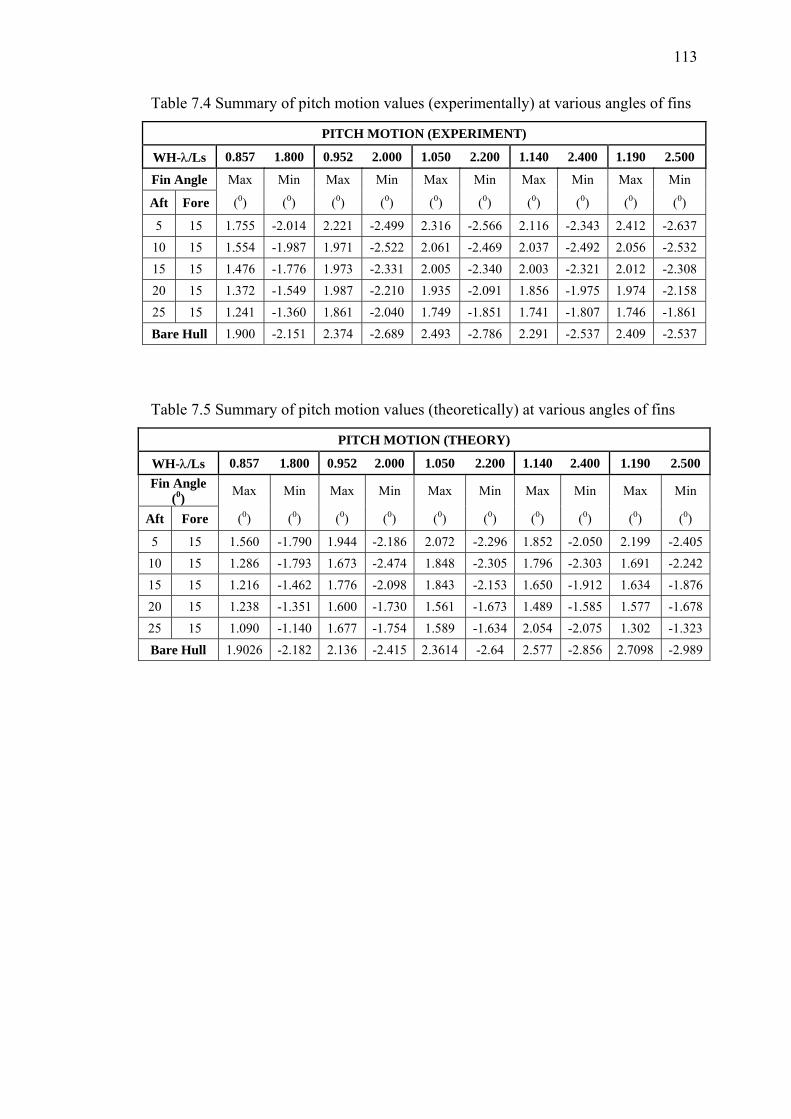
113
Table 7.4 Summary of pitch motion values (experimentally) at various angles of fins
PITCH MOTION (EXPERIMENT)
WH-λ/Ls 0.857 1.800 0.952 2.000 1.050 2.200 1.140 2.400 1.190 2.500
Fin Angle Max Min Max Min Max Min Max Min Max Min
Aft Fore (0) (0) (0) (0) (0) (0) (0) (0) (0) (0)
5 15 1.755 -2.014 2.221 -2.499 2.316 -2.566 2.116 -2.343 2.412 -2.637 10 15 1.554 -1.987 1.971 -2.522 2.061 -2.469 2.037 -2.492 2.056 -2.532 15 15 1.476 -1.776 1.973 -2.331 2.005 -2.340 2.003 -2.321 2.012 -2.308 20 15 1.372 -1.549 1.987 -2.210 1.935 -2.091 1.856 -1.975 1.974 -2.158 25 15 1.241 -1.360 1.861 -2.040 1.749 -1.851 1.741 -1.807 1.746 -1.861 Bare Hull 1.900 -2.151 2.374 -2.689 2.493 -2.786 2.291 -2.537 2.409 -2.537
Table 7.5 Summary of pitch motion values (theoretically) at various angles of fins
PITCH MOTION (THEORY)
WH-λ/Ls 0.857 1.800 0.952 2.000 1.050 2.200 1.140 2.400 1.190 2.500 Fin Angle
(0) Max Min Max Min Max Min Max Min Max Min
Aft Fore (0) (0) (0) (0) (0) (0) (0) (0) (0) (0)
5 15 1.560 -1.790 1.944 -2.186 2.072 -2.296 1.852 -2.050 2.199 -2.405 10 15 1.286 -1.793 1.673 -2.474 1.848 -2.305 1.796 -2.303 1.691 -2.242 15 15 1.216 -1.462 1.776 -2.098 1.843 -2.153 1.650 -1.912 1.634 -1.876 20 15 1.238 -1.351 1.600 -1.730 1.561 -1.673 1.489 -1.585 1.577 -1.678 25 15 1.090 -1.140 1.677 -1.754 1.589 -1.634 2.054 -2.075 1.302 -1.323 Bare Hull 1.9026 -2.182 2.136 -2.415 2.3614 -2.64 2.577 -2.856 2.7098 -2.989
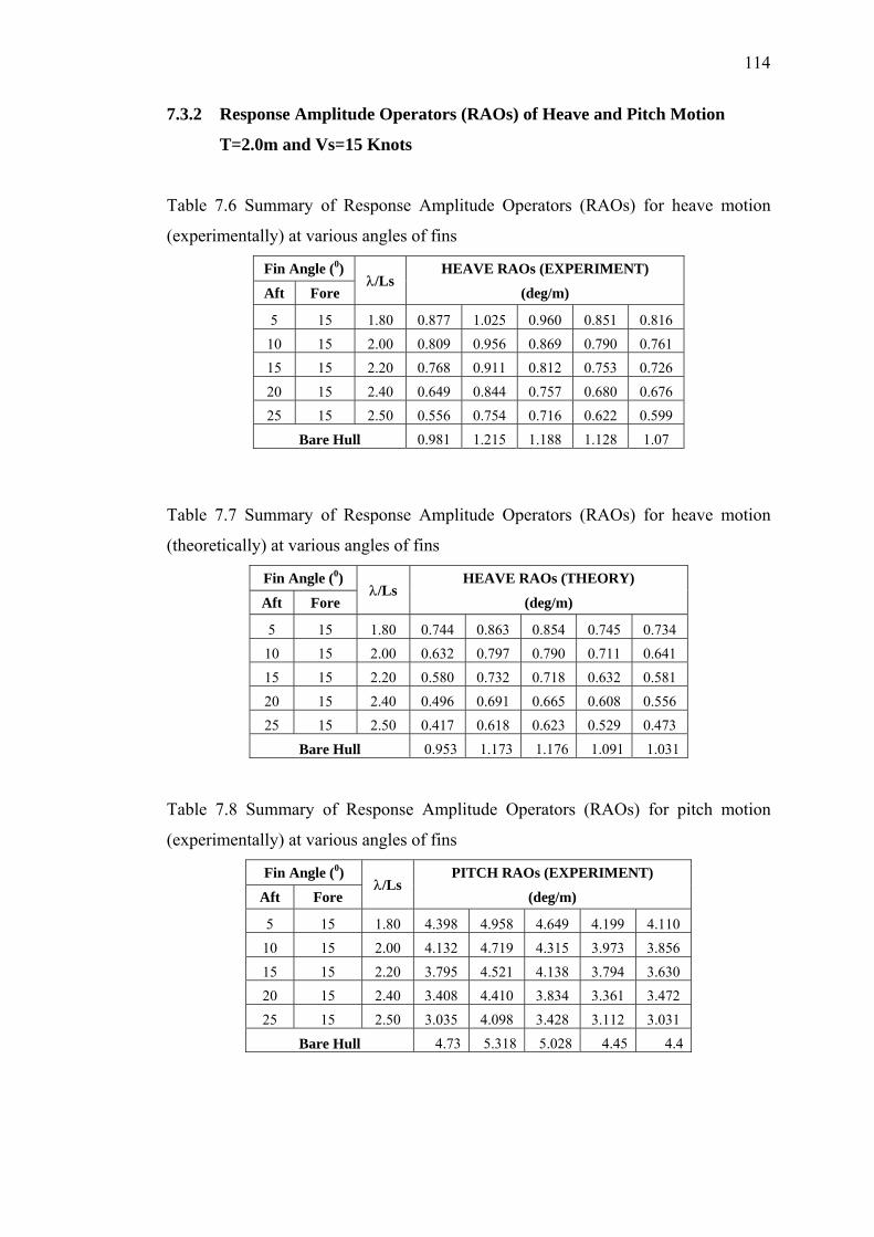
114
7.3.2 Response Amplitude Operators (RAOs) of Heave and Pitch Motion
T=2.0m and Vs=15 Knots
Table 7.6 Summary of Response Amplitude Operators (RAOs) for heave motion
(experimentally) at various angles of fins
Fin Angle (0) HEAVE RAOs (EXPERIMENT)
Aft Fore λ/Ls
(deg/m)
5 15 1.80 0.877 1.025 0.960 0.851 0.816 10 15 2.00 0.809 0.956 0.869 0.790 0.761 15 15 2.20 0.768 0.911 0.812 0.753 0.726 20 15 2.40 0.649 0.844 0.757 0.680 0.676 25 15 2.50 0.556 0.754 0.716 0.622 0.599
Bare Hull 0.981 1.215 1.188 1.128 1.07
Table 7.7 Summary of Response Amplitude Operators (RAOs) for heave motion
(theoretically) at various angles of fins
Fin Angle (0) HEAVE RAOs (THEORY)
Aft Fore λ/Ls
(deg/m)
5 15 1.80 0.744 0.863 0.854 0.745 0.734 10 15 2.00 0.632 0.797 0.790 0.711 0.641 15 15 2.20 0.580 0.732 0.718 0.632 0.581 20 15 2.40 0.496 0.691 0.665 0.608 0.556 25 15 2.50 0.417 0.618 0.623 0.529 0.473
Bare Hull 0.953 1.173 1.176 1.091 1.031 Table 7.8 Summary of Response Amplitude Operators (RAOs) for pitch motion
(experimentally) at various angles of fins
Fin Angle (0) PITCH RAOs (EXPERIMENT)
Aft Fore λ/Ls
(deg/m)
5 15 1.80 4.398 4.958 4.649 4.199 4.110 10 15 2.00 4.132 4.719 4.315 3.973 3.856 15 15 2.20 3.795 4.521 4.138 3.794 3.630 20 15 2.40 3.408 4.410 3.834 3.361 3.472 25 15 2.50 3.035 4.098 3.428 3.112 3.031
Bare Hull 4.73 5.318 5.028 4.45 4.4
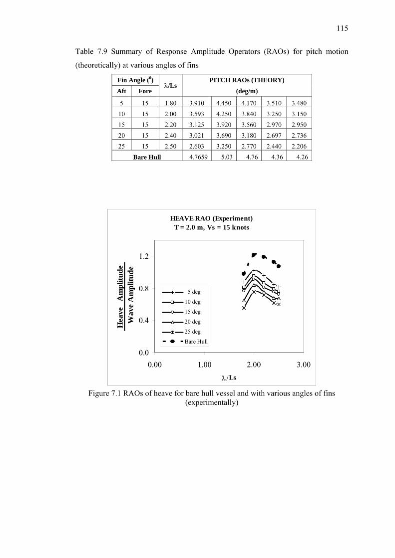
115
Table 7.9 Summary of Response Amplitude Operators (RAOs) for pitch motion
(theoretically) at various angles of fins
Fin Angle (0) PITCH RAOs (THEORY)
Aft Fore λ/Ls
(deg/m)
5 15 1.80 3.910 4.450 4.170 3.510 3.480 10 15 2.00 3.593 4.250 3.840 3.250 3.150 15 15 2.20 3.125 3.920 3.560 2.970 2.950 20 15 2.40 3.021 3.690 3.180 2.697 2.736 25 15 2.50 2.603 3.250 2.770 2.440 2.206
Bare Hull 4.7659 5.03 4.76 4.36 4.26
HEAVE RAO (Experiment)T = 2.0 m, Vs = 15 knots
0.0
0.4
0.8
1.2
0.00 1.00 2.00 3.00
λ/Ls
Hea
ve
Am
plitu
de
Wav
e A
mpl
itude
5 deg
10 deg
15 deg
20 deg
25 deg
Bare Hull
Figure 7.1 RAOs of heave for bare hull vessel and with various angles of fins
(experimentally)
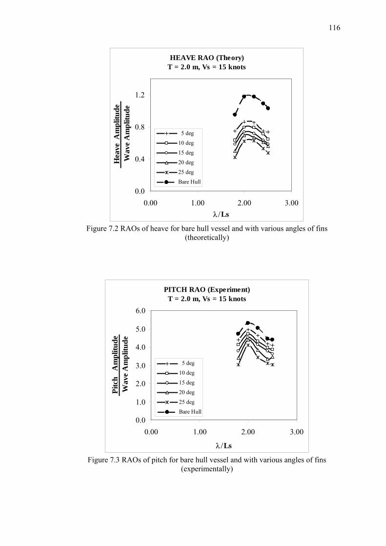
116
HEAVE RAO (Theory)T = 2.0 m, Vs = 15 knots
0.0
0.4
0.8
1.2
0.00 1.00 2.00 3.00λ/Ls
Hea
ve A
mpl
itude
W
ave
Am
plitu
de
5 deg
10 deg
15 deg
20 deg
25 deg
Bare Hull
Figure 7.2 RAOs of heave for bare hull vessel and with various angles of fins
(theoretically)
PITCH RAO (Experiment)T = 2.0 m, Vs = 15 knots
0.0
1.0
2.0
3.0
4.0
5.0
6.0
0.00 1.00 2.00 3.00
λ/Ls
Pitc
h A
mpl
itude
W
ave
Am
plitu
de
5 deg
10 deg
15 deg
20 deg
25 deg
Bare Hull
Figure 7.3 RAOs of pitch for bare hull vessel and with various angles of fins
(experimentally)
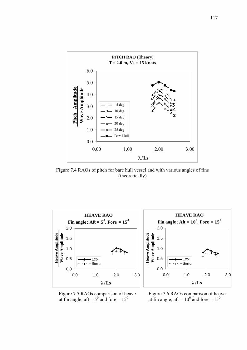
117
Figure 7.4 RAOs of pitch for bare hull vessel and with various angles of fins (theoretically)
HEAVE RAOFin angle; Aft = 50, Fore = 150
0.0
0.5
1.0
1.5
2.0
0.0 1.0 2.0 3.0
λ/Ls
H
eave
Am
plitu
de__
Wav
e A
mpl
itude
ExpSimu
HEAVE RAOFin angle; Aft = 100, Fore = 150
0.0
0.5
1.0
1.5
2.0
0.0 1.0 2.0 3.0
λ/Ls
H
eave
Am
plitu
de__
Wav
e A
mpl
itude
ExpSimu
Figure 7.5 RAOs comparison of heaveat fin angle; aft = 50 and fore = 150
Figure 7.6 RAOs comparison of heaveat fin angle; aft = 100 and fore = 150
PITCH RAO (Theory)T = 2.0 m, Vs = 15 knots
0.0
1.0
2.0
3.0
4.0
5.0
6.0
0.00 1.00 2.00 3.00
λ/Ls
Pitc
h A
mpl
itude
W
ave
Am
plitu
de
5 deg
10 deg
15 deg
20 deg
25 deg
Bare Hull
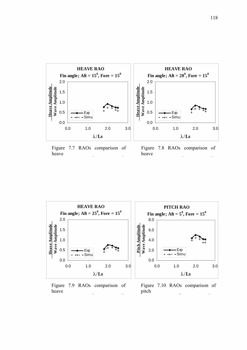
118
HEAVE RAOFin angle; Aft = 150, Fore = 150
0.0
0.5
1.0
1.5
2.0
0.0 1.0 2.0 3.0
λ/Ls
H
eave
Am
plitu
de__
Wav
e A
mpl
itude
ExpSimu
HEAVE RAOFin angle; Aft = 200, Fore = 150
0.0
0.5
1.0
1.5
2.0
0.0 1.0 2.0 3.0
λ/Ls
Hea
ve A
mpl
itude
__W
ave
Am
plitu
de
ExpSimu
Figure 7.7 RAOs comparison of heave
0 0
Figure 7.8 RAOs comparison of heave
0 0
PITCH RAOFin angle; Aft = 50, Fore = 150
0.0
2.0
4.0
6.0
8.0
0.0 1.0 2.0 3.0
λ/Ls
P
itch
Am
plitu
de_
Wav
e A
mpl
itude
ExpSimu
HEAVE RAOFin angle; Aft = 250, Fore = 150
0.0
0.5
1.0
1.5
2.0
0.0 1.0 2.0 3.0
λ/Ls
H
eave
Am
plitu
de__
Wav
e A
mpl
itude
ExpSimu
Figure 7.9 RAOs comparison of heave
0 0
Figure 7.10 RAOs comparison of pitch
0 0

119
PITCH RAOFin angle; Aft = 100, Fore = 150
0.0
2.0
4.0
6.0
8.0
0.0 1.0 2.0 3.0
λ/Ls
P
itch
Am
plitu
de_
Wav
e A
mpl
itude
ExpSimu
PITCH RAOFin angle; Aft = 150, Fore = 150
0.0
2.0
4.0
6.0
8.0
0.0 1.0 2.0 3.0
λ/Ls
Pitc
h A
mpl
itude
_W
ave
Am
plitu
de
ExpSimu
Figure 7.11 RAOs comparison of heave
0 0
Figure 7.12 RAOs comparison of pitch
0 0
PITCH RAOFin angle; Aft = 200, Fore = 150
0.0
2.0
4.0
6.0
8.0
0.0 1.0 2.0 3.0
λ/Ls
P
itch
Am
plitu
de_
Wav
e A
mpl
itude
ExpSimu
PITCH RAOFin angle; Aft = 250, Fore = 150
0.0
2.0
4.0
6.0
8.0
0.0 1.0 2.0 3.0
λ/Ls
P
itch
Am
plitu
de_
Wav
e A
mpl
itude
ExpSimu
Figure 7.13 RAOs comparison of pitch
Figure 7.14 RAOs comparison of pitch
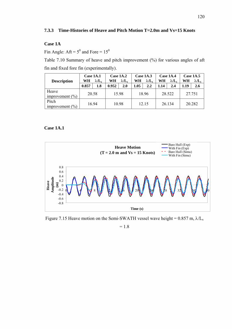
120
7.3.3 Time-Histories of Heave and Pitch Motion T=2.0m and Vs=15 Knots
Case 1A
Fin Angle: Aft = 50 and Fore = 150
Table 7.10 Summary of heave and pitch improvement (%) for various angles of aft
fin and fixed fore fin (experimentally). Case 1A.1 WH λ/Ls
Case 1A.2 WH λ/Ls
Case 1A.3 WH λ/Ls
Case 1A.4 WH λ/Ls
Case 1A.5 WH λ/Ls Description
0.857 1.8 0.952 2.0 1.05 2.2 1.14 2.4 1.19 2.6 Heave improvement (%) 20.58 15.98 18.96 28.522 27.751
Pitch improvement (%) 16.94 10.98 12.15 26.134 20.282
Case 1A.1
Heave Motion(T = 2.0 m and Vs = 15 Knots)
-0.8-0.6-0.4-0.2
00.20.40.60.8
0 4 8 12 16 20 24 28 32 36 40
Time (s)
Hea
ve
Am
plitu
de(m
)
Bare Hull (Exp)With Fin (Exp)Bare Hull (Simu)With Fin (Simu)
Figure 7.15 Heave motion on the Semi-SWATH vessel wave height = 0.857 m, λ/Ls
= 1.8
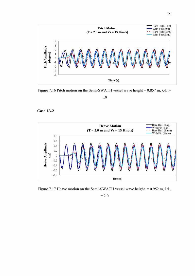
121
Pitch Motion(T = 2.0 m and Vs = 15 Knots)
-4-3-2-101234
0 4 8 12 16 20 24 28 32 36 40
Time (s)
Pitc
h A
mpl
itude
(deg
ree)
Bare Hull (Exp)With Fin (Exp)Bare Hull (Simu)With Fin (Simu)
Figure 7.16 Pitch motion on the Semi-SWATH vessel wave height = 0.857 m, λ/Ls =
1.8
Case 1A.2
Heave Motion(T = 2.0 m and Vs = 15 Knots)
-0.8
-0.6
-0.4
-0.2
0
0.2
0.4
0.6
0.8
0 4 8 12 16 20 24 28 32 36 40
Time (s)
Hea
ve A
mpl
itude
(m)
Bare Hull (Exp)With Fin (Exp)Bare Hull (Simu)With Fin (Simu)
Figure 7.17 Heave motion on the Semi-SWATH vessel wave height = 0.952 m, λ/Ls
= 2.0
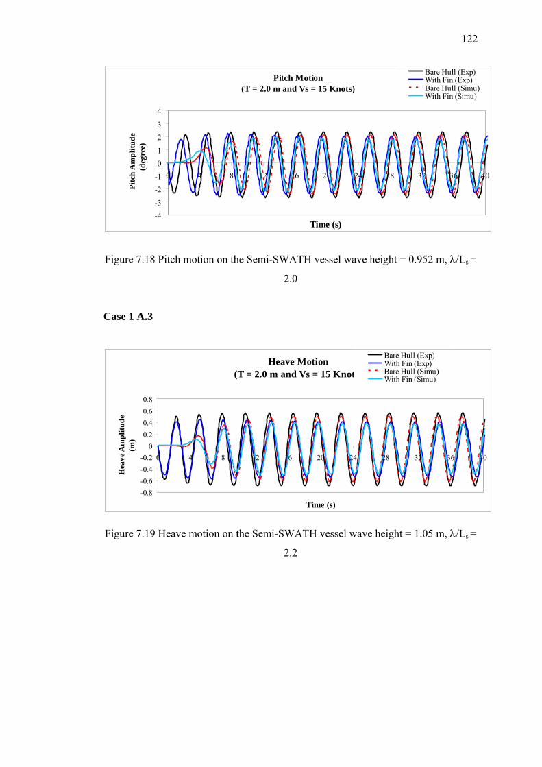
122
Pitch Motion(T = 2.0 m and Vs = 15 Knots)
-4-3
-2-1
01
23
4
0 4 8 12 16 20 24 28 32 36 40
Time (s)
Pitc
h A
mpl
itude
(deg
ree)
Bare Hull (Exp)With Fin (Exp)Bare Hull (Simu)With Fin (Simu)
Figure 7.18 Pitch motion on the Semi-SWATH vessel wave height = 0.952 m, λ/Ls =
2.0
Case 1 A.3
Heave Motion(T = 2.0 m and Vs = 15 Knots)
-0.8-0.6-0.4-0.2
00.20.40.60.8
0 4 8 12 16 20 24 28 32 36 40
Time (s)
Hea
ve A
mpl
itude
(m)
Bare Hull (Exp)With Fin (Exp)Bare Hull (Simu)With Fin (Simu)
Figure 7.19 Heave motion on the Semi-SWATH vessel wave height = 1.05 m, λ/Ls =
2.2
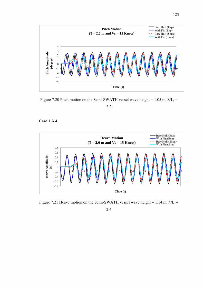
123
Pitch Motion(T = 2.0 m and Vs = 15 Knots)
-4-3-2-101234
0 4 8 12 16 20 24 28 32 36 40
Time (s)
Pitc
h A
mpl
itude
(deg
ree)
Bare Hull (Exp)With Fin (Exp)Bare Hull (Simu)With Fin (Simu)
Figure 7.20 Pitch motion on the Semi-SWATH vessel wave height = 1.05 m, λ/Ls =
2.2
Case 1 A.4
Heave Motion(T = 2.0 m and Vs = 15 Knots)
-0.8
-0.6
-0.4
-0.2
0
0.2
0.4
0.6
0.8
0 4 8 12 16 20 24 28 32 36 40
Time (s)
Hea
ve A
mpl
itude
(m)
Bare Hull (Exp)With Fin (Exp)Bare Hull (Simu)With Fin (Simu)
Figure 7.21 Heave motion on the Semi-SWATH vessel wave height = 1.14 m, λ/Ls =
2.4
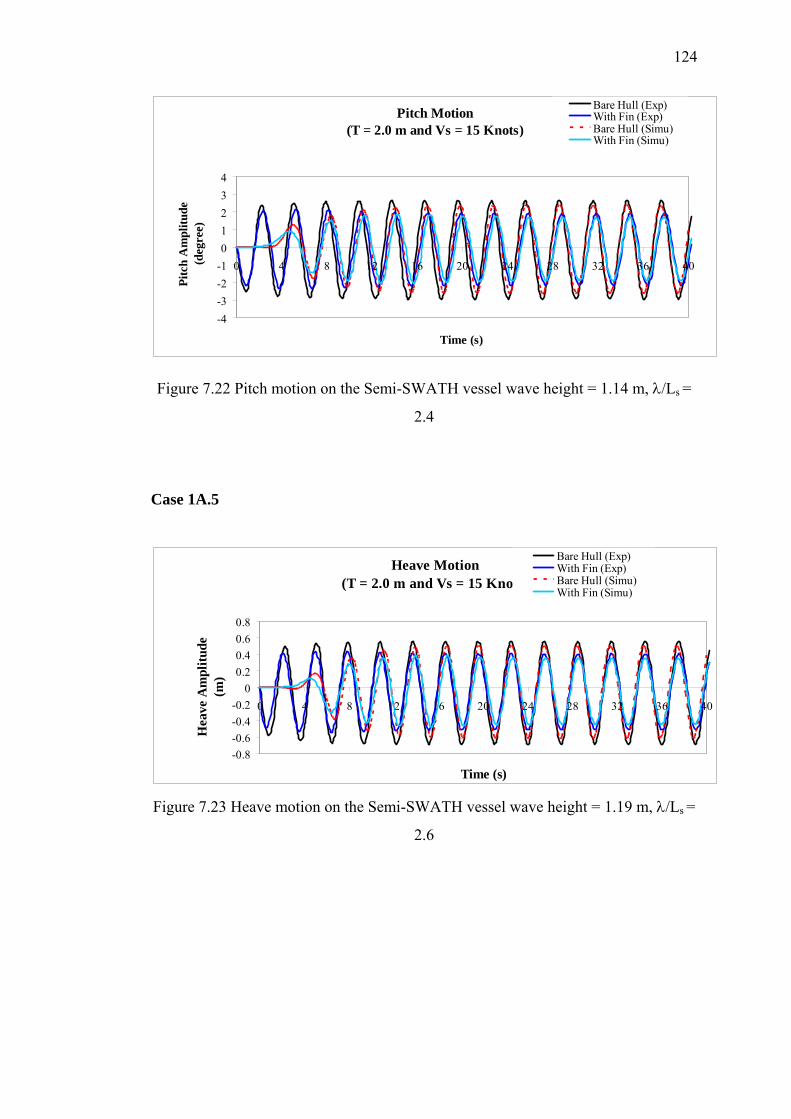
124
Pitch Motion(T = 2.0 m and Vs = 15 Knots)
-4-3-2-101234
0 4 8 12 16 20 24 28 32 36 40
Time (s)
Pitc
h A
mpl
itude
(deg
ree)
Bare Hull (Exp)With Fin (Exp)Bare Hull (Simu)With Fin (Simu)
Figure 7.22 Pitch motion on the Semi-SWATH vessel wave height = 1.14 m, λ/Ls =
2.4
Case 1A.5
Heave Motion(T = 2.0 m and Vs = 15 Knots)
-0.8-0.6-0.4-0.2
00.20.40.60.8
0 4 8 12 16 20 24 28 32 36 40
Time (s)
Hea
ve A
mpl
itude
(m)
Bare Hull (Exp)With Fin (Exp)Bare Hull (Simu)With Fin (Simu)
Figure 7.23 Heave motion on the Semi-SWATH vessel wave height = 1.19 m, λ/Ls =
2.6
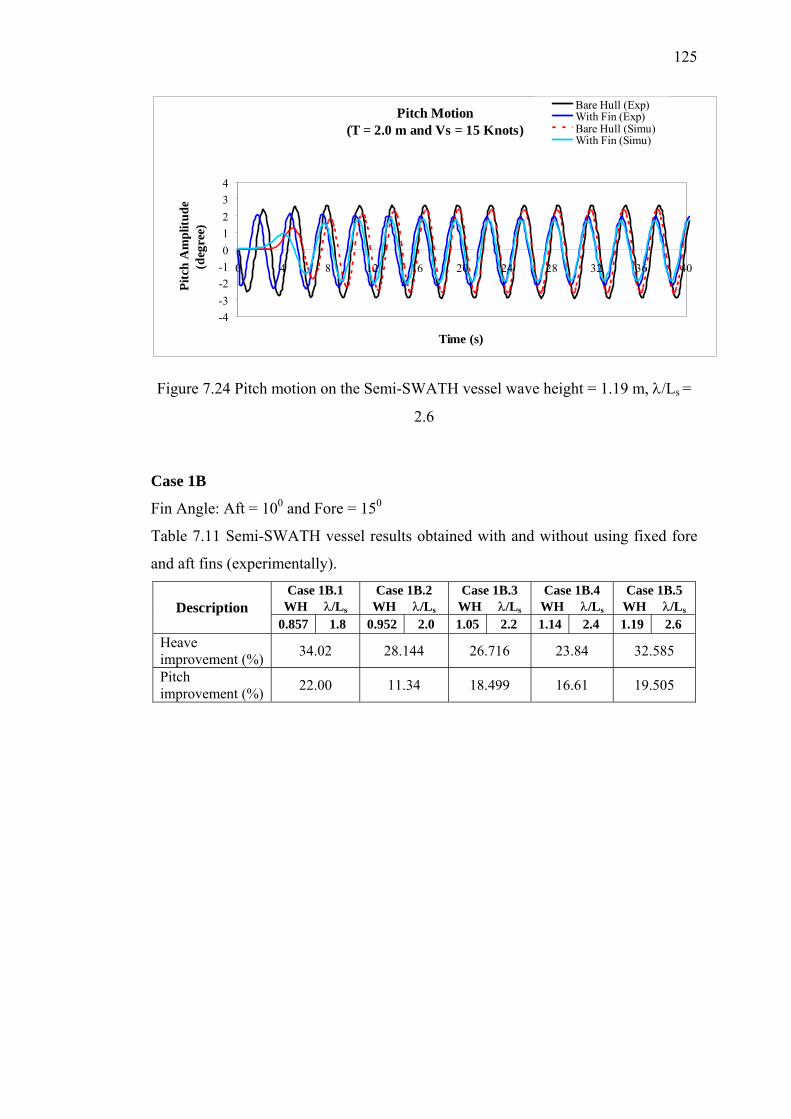
125
Pitch Motion(T = 2.0 m and Vs = 15 Knots)
-4-3-2-101234
0 4 8 12 16 20 24 28 32 36 40
Time (s)
Pitc
h A
mpl
itude
(deg
ree)
Bare Hull (Exp)With Fin (Exp)Bare Hull (Simu)With Fin (Simu)
Figure 7.24 Pitch motion on the Semi-SWATH vessel wave height = 1.19 m, λ/Ls =
2.6
Case 1B
Fin Angle: Aft = 100 and Fore = 150
Table 7.11 Semi-SWATH vessel results obtained with and without using fixed fore
and aft fins (experimentally). Case 1B.1
WH λ/Ls Case 1B.2
WH λ/Ls Case 1B.3
WH λ/Ls Case 1B.4
WH λ/Ls Case 1B.5
WH λ/Ls Description 0.857 1.8 0.952 2.0 1.05 2.2 1.14 2.4 1.19 2.6
Heave improvement (%) 34.02 28.144 26.716 23.84 32.585
Pitch improvement (%) 22.00 11.34 18.499 16.61 19.505
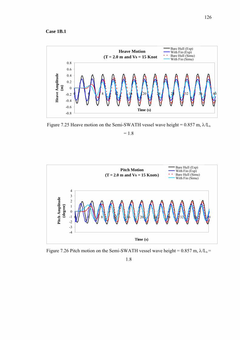
126
Case 1B.1
Heave Motion(T = 2.0 m and Vs = 15 Knots)
-0.8
-0.6
-0.4
-0.2
0
0.2
0.4
0.6
0.8
0 4 8 12 16 20 24 28 32 36 40
Time (s)
Hea
ve A
mpl
itude
(m)
Bare Hull (Exp)With Fin (Exp)Bare Hull (Simu)With Fin (Simu)
Figure 7.25 Heave motion on the Semi-SWATH vessel wave height = 0.857 m, λ/Ls
= 1.8
Pitch Motion(T = 2.0 m and Vs = 15 Knots)
-4-3-2-101234
0 4 8 12 16 20 24 28 32 36 40
Time (s)
Pitc
h A
mpl
itude
(deg
ree)
Bare Hull (Exp)With Fin (Exp)Bare Hull (Simu)With Fin (Simu)
Figure 7.26 Pitch motion on the Semi-SWATH vessel wave height = 0.857 m, λ/Ls =
1.8
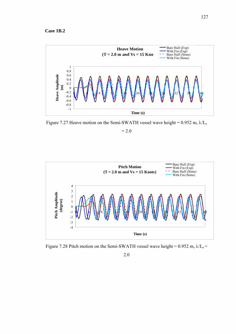
127
Case 1B.2
Heave Motion(T = 2.0 m and Vs = 15 Knots)
-1-0.8-0.6-0.4-0.2
00.20.40.60.8
1
0 4 8 12 16 20 24 28 32 36 40
Time (s)
Hea
ve A
mpl
itude
(m)
Bare Hull (Exp)With Fin (Exp)Bare Hull (Simu)With Fin (Simu)
Figure 7.27 Heave motion on the Semi-SWATH vessel wave height = 0.952 m, λ/Ls
= 2.0
Pitch Motion(T = 2.0 m and Vs = 15 Knots)
-4-3-2-101234
0 4 8 12 16 20 24 28 32 36 40
Time (s)
Pitc
h A
mpl
itude
(deg
ree)
Bare Hull (Exp)With Fin (Exp)Bare Hull (Simu)With Fin (Simu)
Figure 7.28 Pitch motion on the Semi-SWATH vessel wave height = 0.952 m, λ/Ls =
2.0
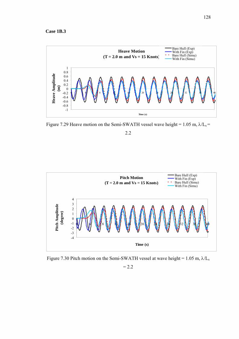
128
Case 1B.3
Heave Motion(T = 2.0 m and Vs = 15 Knots)
-1-0.8-0.6-0.4-0.2
00.20.40.60.8
1
0 4 8 12 16 20 24 28 32 36 40
Time (s)
Hea
ve A
mpl
itude
(m)
Bare Hull (Exp)With Fin (Exp)Bare Hull (Simu)With Fin (Simu)
Figure 7.29 Heave motion on the Semi-SWATH vessel wave height = 1.05 m, λ/Ls =
2.2
Pitch Motion(T = 2.0 m and Vs = 15 Knots)
-4-3-2-101234
0 4 8 12 16 20 24 28 32 36 40
Time (s)
Pitc
h A
mpl
itude
(deg
ree)
Bare Hull (Exp)With Fin (Exp)Bare Hull (Simu)With Fin (Simu)
Figure 7.30 Pitch motion on the Semi-SWATH vessel at wave height = 1.05 m, λ/Ls
= 2.2
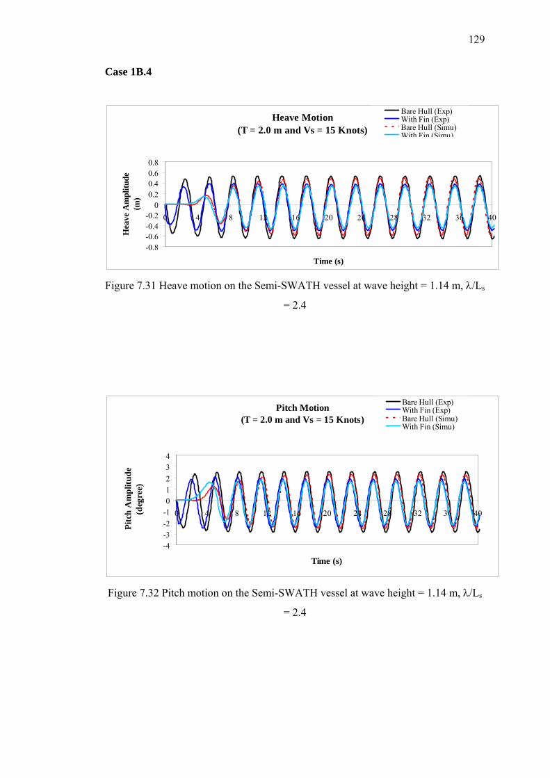
129
Case 1B.4
Heave Motion(T = 2.0 m and Vs = 15 Knots)
-0.8-0.6-0.4-0.2
00.20.40.60.8
0 4 8 12 16 20 24 28 32 36 40
Time (s)
Hea
ve A
mpl
itude
(m)
Bare Hull (Exp)With Fin (Exp)Bare Hull (Simu)With Fin (Simu)
Figure 7.31 Heave motion on the Semi-SWATH vessel at wave height = 1.14 m, λ/Ls
= 2.4
Pitch Motion(T = 2.0 m and Vs = 15 Knots)
-4-3-2-101234
0 4 8 12 16 20 24 28 32 36 40
Time (s)
Pitc
h A
mpl
itude
(deg
ree)
Bare Hull (Exp)With Fin (Exp)Bare Hull (Simu)With Fin (Simu)
Figure 7.32 Pitch motion on the Semi-SWATH vessel at wave height = 1.14 m, λ/Ls
= 2.4
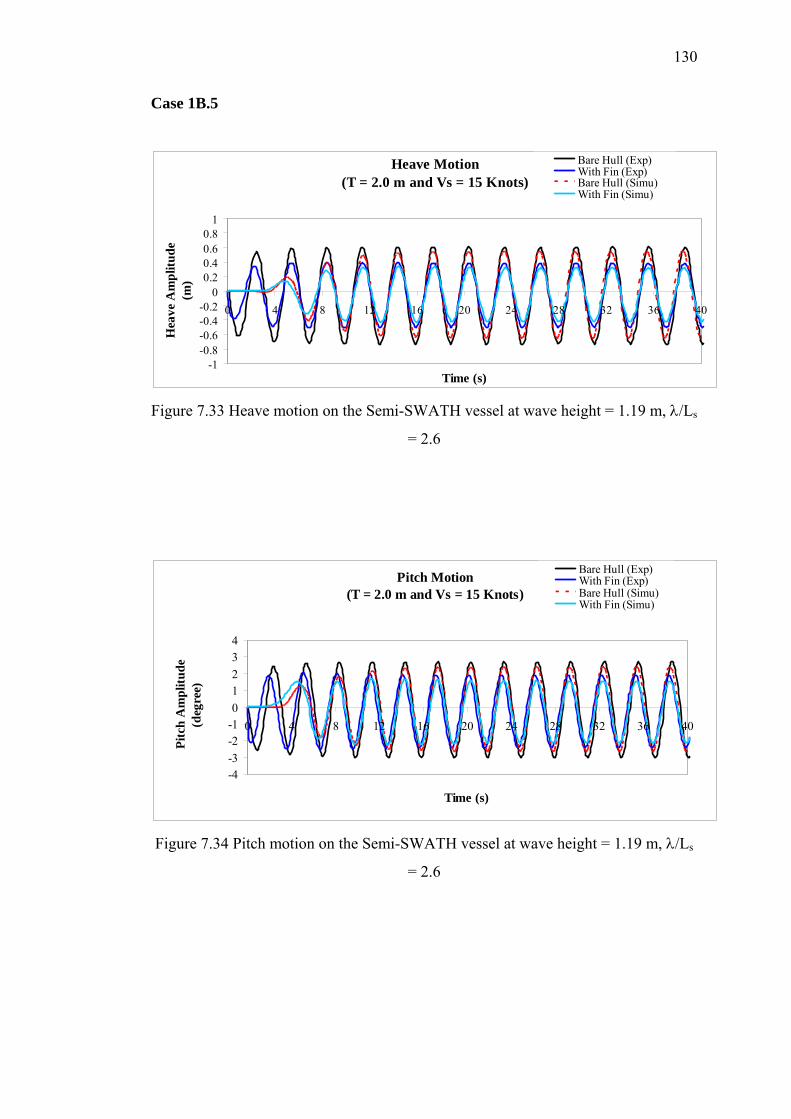
130
Case 1B.5
Heave Motion(T = 2.0 m and Vs = 15 Knots)
-1-0.8-0.6-0.4-0.2
00.20.40.60.8
1
0 4 8 12 16 20 24 28 32 36 40
Time (s)
Hea
ve A
mpl
itude
(m)
Bare Hull (Exp)With Fin (Exp)Bare Hull (Simu)With Fin (Simu)
Figure 7.33 Heave motion on the Semi-SWATH vessel at wave height = 1.19 m, λ/Ls
= 2.6
Pitch Motion(T = 2.0 m and Vs = 15 Knots)
-4-3-2-101234
0 4 8 12 16 20 24 28 32 36 40
Time (s)
Pitc
h A
mpl
itude
(deg
ree)
Bare Hull (Exp)With Fin (Exp)Bare Hull (Simu)With Fin (Simu)
Figure 7.34 Pitch motion on the Semi-SWATH vessel at wave height = 1.19 m, λ/Ls
= 2.6
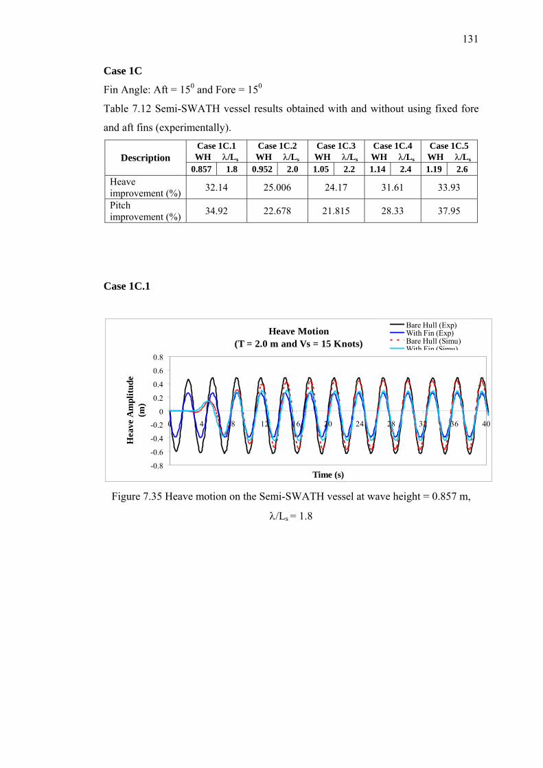
131
Case 1C
Fin Angle: Aft = 150 and Fore = 150
Table 7.12 Semi-SWATH vessel results obtained with and without using fixed fore
and aft fins (experimentally). Case 1C.1 WH λ/Ls
Case 1C.2 WH λ/Ls
Case 1C.3 WH λ/Ls
Case 1C.4 WH λ/Ls
Case 1C.5 WH λ/Ls Description
0.857 1.8 0.952 2.0 1.05 2.2 1.14 2.4 1.19 2.6 Heave improvement (%) 32.14 25.006 24.17 31.61 33.93
Pitch improvement (%) 34.92 22.678 21.815 28.33 37.95
Case 1C.1
Heave Motion(T = 2.0 m and Vs = 15 Knots)
-0.8
-0.6
-0.4
-0.2
0
0.2
0.4
0.6
0.8
0 4 8 12 16 20 24 28 32 36 40
Time (s)
Hea
ve A
mpl
itude
(m)
Bare Hull (Exp)With Fin (Exp)Bare Hull (Simu)With Fin (Simu)
Figure 7.35 Heave motion on the Semi-SWATH vessel at wave height = 0.857 m,
λ/Ls = 1.8
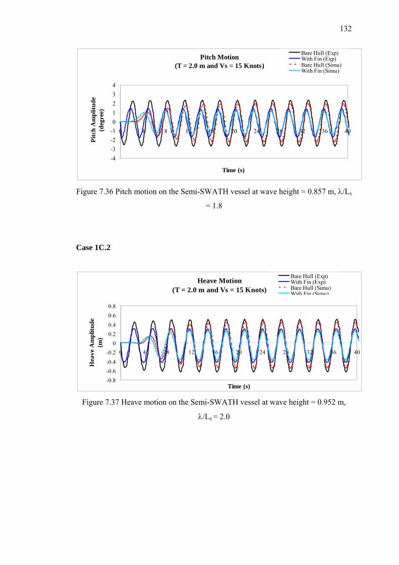
132
Pitch Motion(T = 2.0 m and Vs = 15 Knots)
-4-3-2-101234
0 4 8 12 16 20 24 28 32 36 40
Time (s)
Pitc
h A
mpl
itude
(deg
ree)
Bare Hull (Exp)With Fin (Exp)Bare Hull (Simu)With Fin (Simu)
Figure 7.36 Pitch motion on the Semi-SWATH vessel at wave height = 0.857 m, λ/Ls
= 1.8
Case 1C.2
Heave Motion(T = 2.0 m and Vs = 15 Knots)
-0.8-0.6-0.4-0.2
00.20.40.60.8
0 4 8 12 16 20 24 28 32 36 40
Time (s)
Hea
ve A
mpl
itude
(m)
Bare Hull (Exp)With Fin (Exp)Bare Hull (Simu)With Fin (Simu)
Figure 7.37 Heave motion on the Semi-SWATH vessel at wave height = 0.952 m,
λ/Ls = 2.0
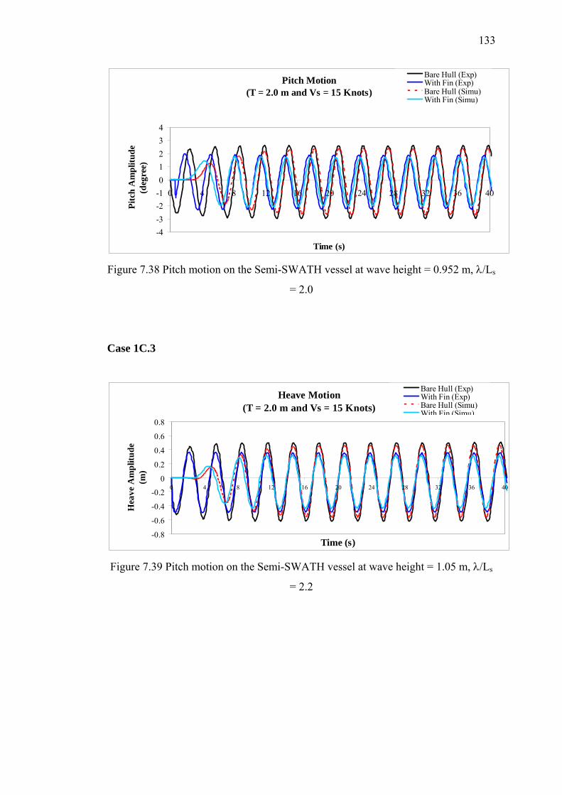
133
Pitch Motion(T = 2.0 m and Vs = 15 Knots)
-4-3-2-101234
0 4 8 12 16 20 24 28 32 36 40
Time (s)
Pitc
h A
mpl
itude
(deg
ree)
Bare Hull (Exp)With Fin (Exp)Bare Hull (Simu)With Fin (Simu)
Figure 7.38 Pitch motion on the Semi-SWATH vessel at wave height = 0.952 m, λ/Ls
= 2.0
Case 1C.3
Heave Motion(T = 2.0 m and Vs = 15 Knots)
-0.8
-0.6
-0.4
-0.2
0
0.2
0.4
0.6
0.8
0 4 8 12 16 20 24 28 32 36 40
Time (s)
Hea
ve A
mpl
itude
(m)
Bare Hull (Exp)With Fin (Exp)Bare Hull (Simu)With Fin (Simu)
Figure 7.39 Pitch motion on the Semi-SWATH vessel at wave height = 1.05 m, λ/Ls
= 2.2
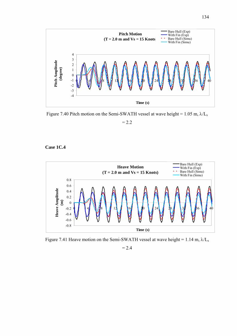
134
Pitch Motion(T = 2.0 m and Vs = 15 Knots)
-4-3-2-101234
0 4 8 12 16 20 24 28 32 36 40
Time (s)
Pitc
h A
mpl
itude
(deg
ree)
Bare Hull (Exp)With Fin (Exp)Bare Hull (Simu)With Fin (Simu)
Figure 7.40 Pitch motion on the Semi-SWATH vessel at wave height = 1.05 m, λ/Ls
= 2.2
Case 1C.4
Heave Motion(T = 2.0 m and Vs = 15 Knots)
-0.8-0.6-0.4-0.2
00.20.40.60.8
0 4 8 12 16 20 24 28 32 36 40
Time (s)
Hea
ve A
mpl
itude
(m)
Bare Hull (Exp)With Fin (Exp)Bare Hull (Simu)With Fin (Simu)
Figure 7.41 Heave motion on the Semi-SWATH vessel at wave height = 1.14 m, λ/Ls
= 2.4
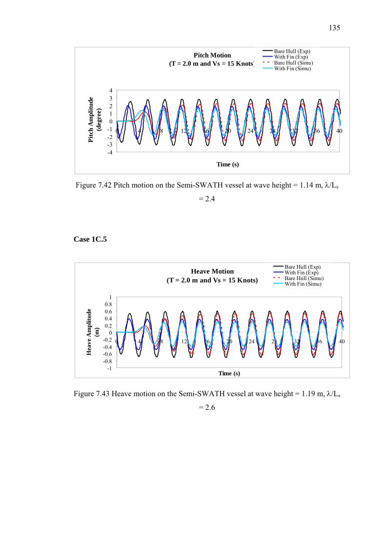
135
Pitch Motion(T = 2.0 m and Vs = 15 Knots)
-4-3-2-101234
0 4 8 12 16 20 24 28 32 36 40
Time (s)
Pitc
h A
mpl
itude
(deg
ree)
Bare Hull (Exp)With Fin (Exp)Bare Hull (Simu)With Fin (Simu)
Figure 7.42 Pitch motion on the Semi-SWATH vessel at wave height = 1.14 m, λ/Ls
= 2.4
Case 1C.5
Heave Motion(T = 2.0 m and Vs = 15 Knots)
-1-0.8-0.6-0.4-0.2
00.20.40.60.8
1
0 4 8 12 16 20 24 28 32 36 40
Time (s)
Hea
ve A
mpl
itude
(m)
Bare Hull (Exp)With Fin (Exp)Bare Hull (Simu)With Fin (Simu)
Figure 7.43 Heave motion on the Semi-SWATH vessel at wave height = 1.19 m, λ/Ls
= 2.6
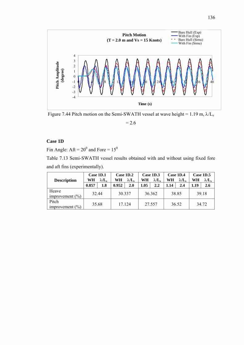
136
Pitch Motion(T = 2.0 m and Vs = 15 Knots)
-4-3-2-101234
0 4 8 12 16 20 24 28 32 36 40
Time (s)
Pitc
h A
mpl
itude
(deg
ree)
Bare Hull (Exp)With Fin (Exp)Bare Hull (Simu)With Fin (Simu)
Figure 7.44 Pitch motion on the Semi-SWATH vessel at wave height = 1.19 m, λ/Ls
= 2.6
Case 1D
Fin Angle: Aft = 200 and Fore = 150
Table 7.13 Semi-SWATH vessel results obtained with and without using fixed fore
and aft fins (experimentally). Case 1D.1 WH λ/Ls
Case 1D.2 WH λ/Ls
Case 1D.3 WH λ/Ls
Case 1D.4 WH λ/Ls
Case 1D.5 WH λ/Ls Description
0.857 1.8 0.952 2.0 1.05 2.2 1.14 2.4 1.19 2.6 Heave improvement (%) 32.44 30.337 36.362 38.85 39.18
Pitch improvement (%) 35.68 17.124 27.557 36.52 34.72
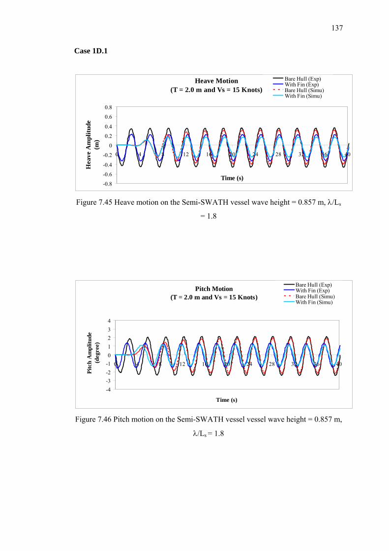
137
Case 1D.1
Heave Motion(T = 2.0 m and Vs = 15 Knots)
-0.8
-0.6
-0.4
-0.2
0
0.2
0.4
0.6
0.8
0 4 8 12 16 20 24 28 32 36 40
Time (s)
Hea
ve A
mpl
itude
(m)
Bare Hull (Exp)With Fin (Exp)Bare Hull (Simu)With Fin (Simu)
Figure 7.45 Heave motion on the Semi-SWATH vessel wave height = 0.857 m, λ/Ls
= 1.8
Pitch Motion(T = 2.0 m and Vs = 15 Knots)
-4-3-2-101234
0 4 8 12 16 20 24 28 32 36 40
Time (s)
Pitc
h A
mpl
itude
(deg
ree)
Bare Hull (Exp)With Fin (Exp)Bare Hull (Simu)With Fin (Simu)
Figure 7.46 Pitch motion on the Semi-SWATH vessel vessel wave height = 0.857 m,
λ/Ls = 1.8
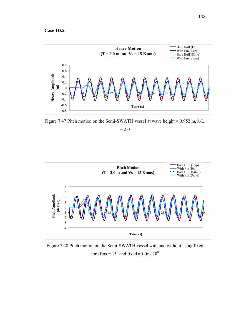
138
Case 1D.2
Heave Motion(T = 2.0 m and Vs = 15 Knots)
-0.8
-0.6
-0.4
-0.2
0
0.2
0.4
0.6
0.8
0 4 8 12 16 20 24 28 32 36 40
Time (s)
Hea
ve A
mpl
itude
(m)
Bare Hull (Exp)With Fin (Exp)Bare Hull (Simu)With Fin (Simu)
Figure 7.47 Pitch motion on the Semi-SWATH vessel at wave height = 0.952 m, λ/Ls
= 2.0
Pitch Motion(T = 2.0 m and Vs = 15 Knots)
-4-3-2-101234
0 4 8 12 16 20 24 28 32 36 40
Time (s)
Pitc
h A
mpl
itude
(deg
ree)
Bare Hull (Exp)With Fin (Exp)Bare Hull (Simu)With Fin (Simu)
Figure 7.48 Pitch motion on the Semi-SWATH vessel with and without using fixed
fore fins = 150 and fixed aft fins 200
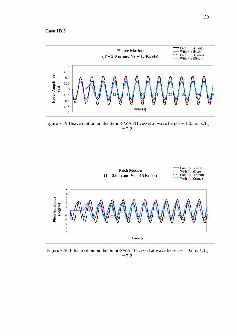
139
Case 1D.3
Heave Motion(T = 2.0 m and Vs = 15 Knots)
-1
-0.75
-0.5
-0.25
0
0.25
0.5
0.75
1
0 4 8 12 16 20 24 28 32 36 40
Time (s)
Hea
ve A
mpl
itude
(m)
Bare Hull (Exp)With Fin (Exp)Bare Hull (Simu)With Fin (Simu)
Figure 7.49 Heave motion on the Semi-SWATH vessel at wave height = 1.05 m, λ/Ls
= 2.2
Pitch Motion(T = 2.0 m and Vs = 15 Knots)
-5-4-3-2-1012345
0 4 8 12 16 20 24 28 32 36 40
Time (s)
Pitc
h A
mpl
itude
(deg
ree)
Bare Hull (Exp)With Fin (Exp)Bare Hull (Simu)With Fin (Simu)
Figure 7.50 Pitch motion on the Semi-SWATH vessel at wave height = 1.05 m, λ/Ls
= 2.2
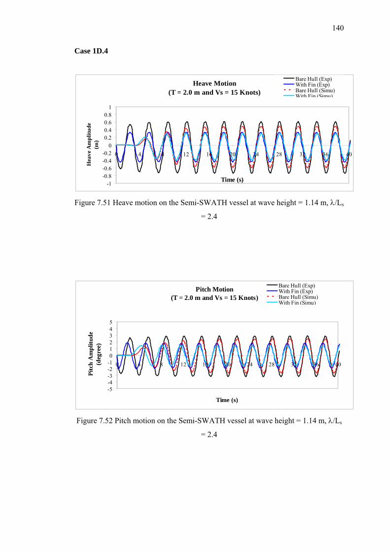
140
Case 1D.4
Heave Motion(T = 2.0 m and Vs = 15 Knots)
-1-0.8-0.6-0.4-0.2
00.20.40.60.8
1
0 4 8 12 16 20 24 28 32 36 40
Time (s)
Hea
ve A
mpl
itude
(m)
Bare Hull (Exp)With Fin (Exp)Bare Hull (Simu)With Fin (Simu)
Figure 7.51 Heave motion on the Semi-SWATH vessel at wave height = 1.14 m, λ/Ls
= 2.4
Pitch Motion(T = 2.0 m and Vs = 15 Knots)
-5-4-3-2-1012345
0 4 8 12 16 20 24 28 32 36 40
Time (s)
Pitc
h A
mpl
itude
(deg
ree)
Bare Hull (Exp)With Fin (Exp)Bare Hull (Simu)With Fin (Simu)
Figure 7.52 Pitch motion on the Semi-SWATH vessel at wave height = 1.14 m, λ/Ls
= 2.4
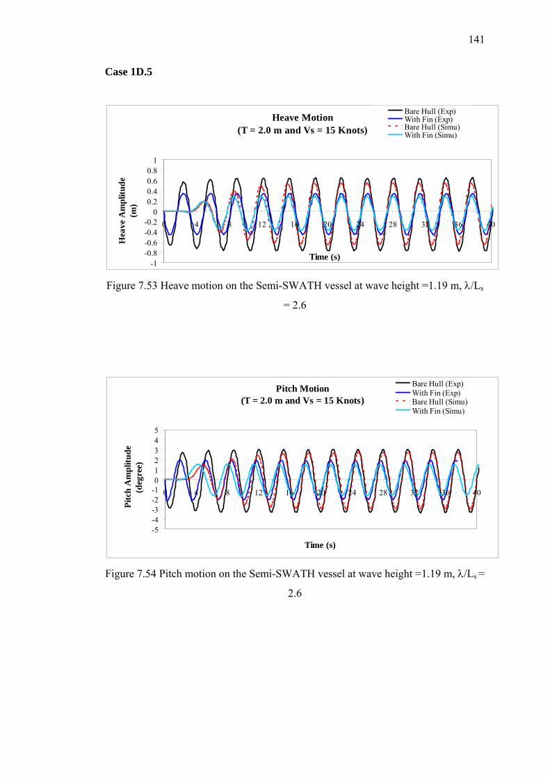
141
Case 1D.5
Heave Motion(T = 2.0 m and Vs = 15 Knots)
-1-0.8-0.6-0.4-0.2
00.20.40.60.8
1
0 4 8 12 16 20 24 28 32 36 40
Time (s)
Hea
ve A
mpl
itude
(m)
Bare Hull (Exp)With Fin (Exp)Bare Hull (Simu)With Fin (Simu)
Figure 7.53 Heave motion on the Semi-SWATH vessel at wave height =1.19 m, λ/Ls
= 2.6
Pitch Motion(T = 2.0 m and Vs = 15 Knots)
-5-4-3-2-1012345
0 4 8 12 16 20 24 28 32 36 40
Time (s)
Pitc
h A
mpl
itude
(deg
ree)
Bare Hull (Exp)With Fin (Exp)Bare Hull (Simu)With Fin (Simu)
Figure 7.54 Pitch motion on the Semi-SWATH vessel at wave height =1.19 m, λ/Ls =
2.6
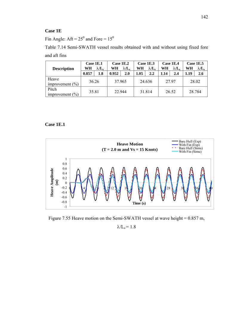
142
Case 1E
Fin Angle: Aft = 250 and Fore = 150
Table 7.14 Semi-SWATH vessel results obtained with and without using fixed fore
and aft fins Case 1E.1
WH λ/Ls Case 1E.2
WH λ/Ls Case 1E.3
WH λ/Ls Case 1E.4
WH λ/Ls Case 1E.5
WH λ/Ls Description 0.857 1.8 0.952 2.0 1.05 2.2 1.14 2.4 1.19 2.6
Heave improvement (%) 36.26 37.965 24.636 27.97 28.02
Pitch improvement (%) 35.81 22.944 31.814 26.52 28.784
Case 1E.1
Heave Motion(T = 2.0 m and Vs = 15 Knots)
-1-0.8-0.6-0.4-0.2
00.20.40.60.8
1
0 4 8 12 16 20 24 28 32 36 40
Time (s)
Hea
ve A
mpl
itude
(m)
Bare Hull (Exp)With Fin (Exp)Bare Hull (Simu)With Fin (Simu)
Figure 7.55 Heave motion on the Semi-SWATH vessel at wave height = 0.857 m,
λ/Ls = 1.8
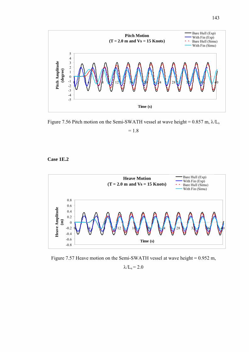
143
Pitch Motion(T = 2.0 m and Vs = 15 Knots)
-5-4-3-2-1012345
0 4 8 12 16 20 24 28 32 36 40
Time (s)
Pitc
h A
mpl
itude
(deg
ree)
Bare Hull (Exp)With Fin (Exp)Bare Hull (Simu)With Fin (Simu)
Figure 7.56 Pitch motion on the Semi-SWATH vessel at wave height = 0.857 m, λ/Ls
= 1.8
Case 1E.2
Heave Motion(T = 2.0 m and Vs = 15 Knots)
-0.8-0.6-0.4-0.2
00.20.40.60.8
0 4 8 12 16 20 24 28 32 36 40
Time (s)
Hea
ve A
mpl
itude
(m)
Bare Hull (Exp)With Fin (Exp)Bare Hull (Simu)With Fin (Simu)
Figure 7.57 Heave motion on the Semi-SWATH vessel at wave height = 0.952 m,
λ/Ls = 2.0
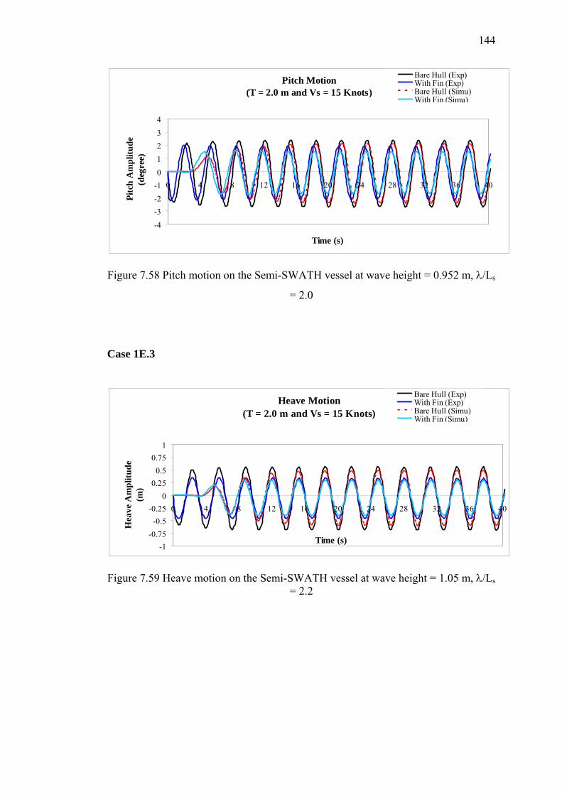
144
Pitch Motion(T = 2.0 m and Vs = 15 Knots)
-4-3-2-101234
0 4 8 12 16 20 24 28 32 36 40
Time (s)
Pitc
h A
mpl
itude
(deg
ree)
Bare Hull (Exp)With Fin (Exp)Bare Hull (Simu)With Fin (Simu)
Figure 7.58 Pitch motion on the Semi-SWATH vessel at wave height = 0.952 m, λ/Ls
= 2.0
Case 1E.3
Heave Motion(T = 2.0 m and Vs = 15 Knots)
-1-0.75
-0.5-0.25
00.25
0.50.75
1
0 4 8 12 16 20 24 28 32 36 40
Time (s)
Hea
ve A
mpl
itude
(m)
Bare Hull (Exp)With Fin (Exp)Bare Hull (Simu)With Fin (Simu)
Figure 7.59 Heave motion on the Semi-SWATH vessel at wave height = 1.05 m, λ/Ls = 2.2
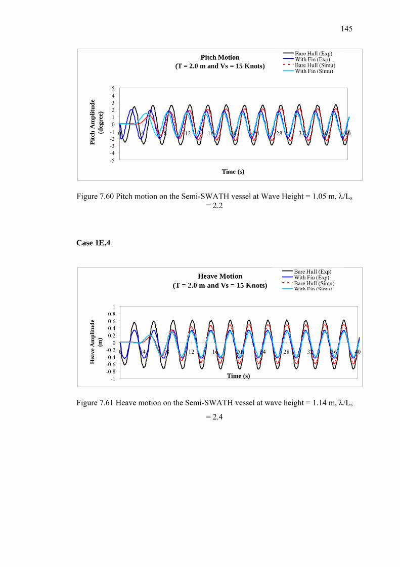
145
Pitch Motion(T = 2.0 m and Vs = 15 Knots)
-5-4-3-2-1012345
0 4 8 12 16 20 24 28 32 36 40
Time (s)
Pitc
h A
mpl
itude
(deg
ree)
Bare Hull (Exp)With Fin (Exp)Bare Hull (Simu)With Fin (Simu)
Figure 7.60 Pitch motion on the Semi-SWATH vessel at Wave Height = 1.05 m, λ/Ls = 2.2
Case 1E.4
Heave Motion(T = 2.0 m and Vs = 15 Knots)
-1-0.8-0.6-0.4-0.2
00.20.40.60.8
1
0 4 8 12 16 20 24 28 32 36 40
Time (s)
Hea
ve A
mpl
itude
(m)
Bare Hull (Exp)With Fin (Exp)Bare Hull (Simu)With Fin (Simu)
Figure 7.61 Heave motion on the Semi-SWATH vessel at wave height = 1.14 m, λ/Ls
= 2.4
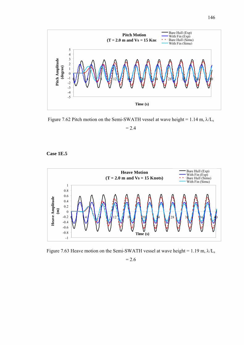
146
Pitch Motion(T = 2.0 m and Vs = 15 Knots)
-5-4-3-2-1012345
0 4 8 12 16 20 24 28 32 36 40
Time (s)
Pitc
h A
mpl
itude
(deg
ree)
Bare Hull (Exp)With Fin (Exp)Bare Hull (Simu)With Fin (Simu)
Figure 7.62 Pitch motion on the Semi-SWATH vessel at wave height = 1.14 m, λ/Ls
= 2.4
Case 1E.5
Heave Motion(T = 2.0 m and Vs = 15 Knots)
-1-0.8-0.6-0.4-0.2
00.20.40.60.8
1
0 4 8 12 16 20 24 28 32 36 40
Time (s)
Hea
ve A
mpl
itude
(m)
Bare Hull (Exp)With Fin (Exp)Bare Hull (Simu)With Fin (Simu)
Figure 7.63 Heave motion on the Semi-SWATH vessel at wave height = 1.19 m, λ/Ls
= 2.6
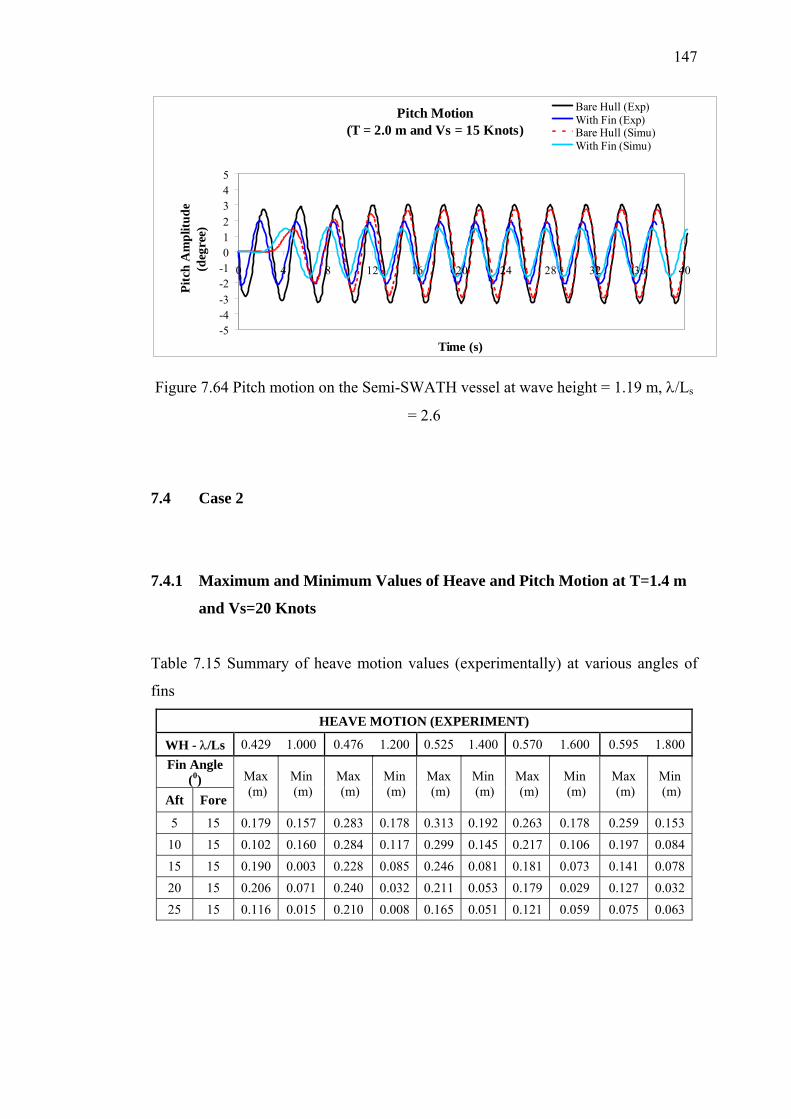
147
Pitch Motion(T = 2.0 m and Vs = 15 Knots)
-5-4-3-2-1012345
0 4 8 12 16 20 24 28 32 36 40
Time (s)
Pitc
h A
mpl
itude
(deg
ree)
Bare Hull (Exp)With Fin (Exp)Bare Hull (Simu)With Fin (Simu)
Figure 7.64 Pitch motion on the Semi-SWATH vessel at wave height = 1.19 m, λ/Ls
= 2.6
7.4 Case 2
7.4.1 Maximum and Minimum Values of Heave and Pitch Motion at T=1.4 m
and Vs=20 Knots
Table 7.15 Summary of heave motion values (experimentally) at various angles of
fins
HEAVE MOTION (EXPERIMENT)
WH - λ/Ls 0.429 1.000 0.476 1.200 0.525 1.400 0.570 1.600 0.595 1.800Fin Angle
(0) Aft Fore
Max (m)
Min (m)
Max (m)
Min (m)
Max (m)
Min (m)
Max (m)
Min (m)
Max (m)
Min (m)
5 15 0.179 0.157 0.283 0.178 0.313 0.192 0.263 0.178 0.259 0.153 10 15 0.102 0.160 0.284 0.117 0.299 0.145 0.217 0.106 0.197 0.084 15 15 0.190 0.003 0.228 0.085 0.246 0.081 0.181 0.073 0.141 0.078 20 15 0.206 0.071 0.240 0.032 0.211 0.053 0.179 0.029 0.127 0.032 25 15 0.116 0.015 0.210 0.008 0.165 0.051 0.121 0.059 0.075 0.063
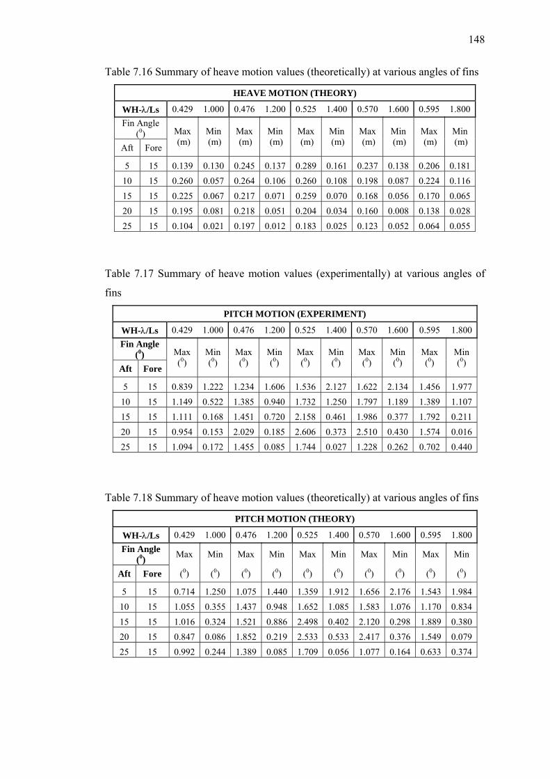
148
Table 7.16 Summary of heave motion values (theoretically) at various angles of fins
HEAVE MOTION (THEORY)
WH-λ/Ls 0.429 1.000 0.476 1.200 0.525 1.400 0.570 1.600 0.595 1.800Fin Angle
(0) Aft Fore
Max (m)
Min (m)
Max (m)
Min (m)
Max (m)
Min (m)
Max (m)
Min (m)
Max (m)
Min (m)
5 15 0.139 0.130 0.245 0.137 0.289 0.161 0.237 0.138 0.206 0.181 10 15 0.260 0.057 0.264 0.106 0.260 0.108 0.198 0.087 0.224 0.116 15 15 0.225 0.067 0.217 0.071 0.259 0.070 0.168 0.056 0.170 0.065 20 15 0.195 0.081 0.218 0.051 0.204 0.034 0.160 0.008 0.138 0.028 25 15 0.104 0.021 0.197 0.012 0.183 0.025 0.123 0.052 0.064 0.055
Table 7.17 Summary of heave motion values (experimentally) at various angles of
fins
PITCH MOTION (EXPERIMENT)
WH-λ/Ls 0.429 1.000 0.476 1.200 0.525 1.400 0.570 1.600 0.595 1.800Fin Angle
(0) Aft Fore
Max (0)
Min (0)
Max (0)
Min (0)
Max (0)
Min (0)
Max (0)
Min (0)
Max (0)
Min (0)
5 15 0.839 1.222 1.234 1.606 1.536 2.127 1.622 2.134 1.456 1.977 10 15 1.149 0.522 1.385 0.940 1.732 1.250 1.797 1.189 1.389 1.107 15 15 1.111 0.168 1.451 0.720 2.158 0.461 1.986 0.377 1.792 0.211 20 15 0.954 0.153 2.029 0.185 2.606 0.373 2.510 0.430 1.574 0.016 25 15 1.094 0.172 1.455 0.085 1.744 0.027 1.228 0.262 0.702 0.440
Table 7.18 Summary of heave motion values (theoretically) at various angles of fins
PITCH MOTION (THEORY)
WH-λ/Ls 0.429 1.000 0.476 1.200 0.525 1.400 0.570 1.600 0.595 1.800Fin Angle
(0) Max Min Max Min Max Min Max Min Max Min
Aft Fore (0) (0) (0) (0) (0) (0) (0) (0) (0) (0)
5 15 0.714 1.250 1.075 1.440 1.359 1.912 1.656 2.176 1.543 1.984 10 15 1.055 0.355 1.437 0.948 1.652 1.085 1.583 1.076 1.170 0.834 15 15 1.016 0.324 1.521 0.886 2.498 0.402 2.120 0.298 1.889 0.380 20 15 0.847 0.086 1.852 0.219 2.533 0.533 2.417 0.376 1.549 0.079 25 15 0.992 0.244 1.389 0.085 1.709 0.056 1.077 0.164 0.633 0.374
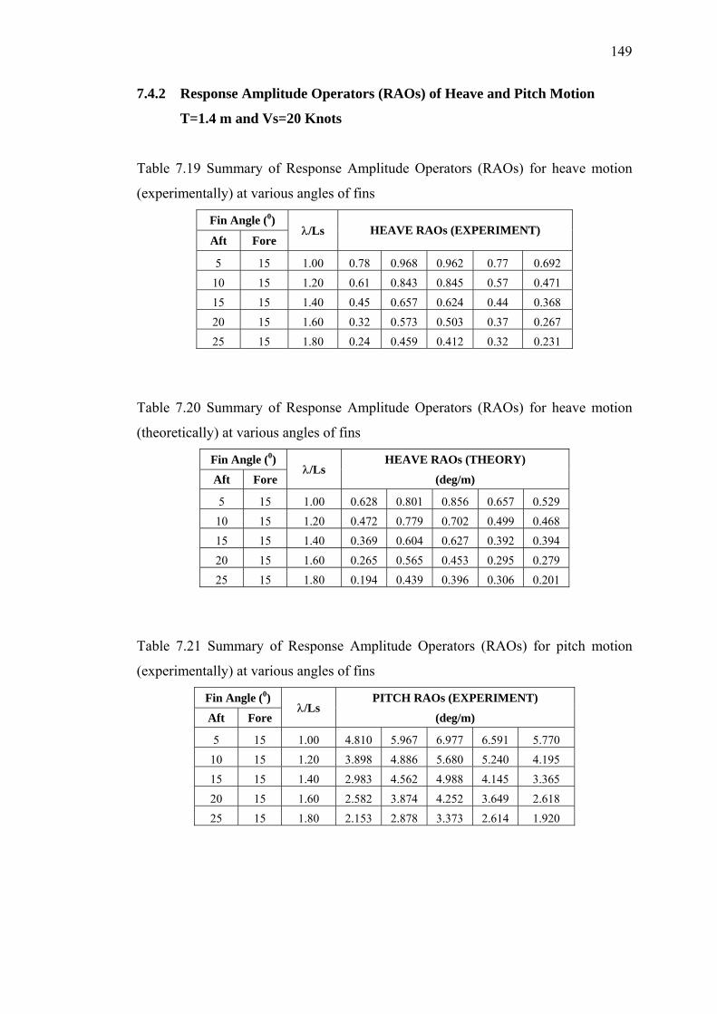
149
7.4.2 Response Amplitude Operators (RAOs) of Heave and Pitch Motion
T=1.4 m and Vs=20 Knots
Table 7.19 Summary of Response Amplitude Operators (RAOs) for heave motion
(experimentally) at various angles of fins
Fin Angle (0)
Aft Fore λ/Ls HEAVE RAOs (EXPERIMENT)
5 15 1.00 0.78 0.968 0.962 0.77 0.692 10 15 1.20 0.61 0.843 0.845 0.57 0.471 15 15 1.40 0.45 0.657 0.624 0.44 0.368 20 15 1.60 0.32 0.573 0.503 0.37 0.267 25 15 1.80 0.24 0.459 0.412 0.32 0.231
Table 7.20 Summary of Response Amplitude Operators (RAOs) for heave motion
(theoretically) at various angles of fins
Fin Angle (0) HEAVE RAOs (THEORY)
Aft Fore λ/Ls
(deg/m)
5 15 1.00 0.628 0.801 0.856 0.657 0.529 10 15 1.20 0.472 0.779 0.702 0.499 0.468 15 15 1.40 0.369 0.604 0.627 0.392 0.394 20 15 1.60 0.265 0.565 0.453 0.295 0.279 25 15 1.80 0.194 0.439 0.396 0.306 0.201
Table 7.21 Summary of Response Amplitude Operators (RAOs) for pitch motion
(experimentally) at various angles of fins
Fin Angle (0) PITCH RAOs (EXPERIMENT)
Aft Fore λ/Ls
(deg/m)
5 15 1.00 4.810 5.967 6.977 6.591 5.770 10 15 1.20 3.898 4.886 5.680 5.240 4.195 15 15 1.40 2.983 4.562 4.988 4.145 3.365 20 15 1.60 2.582 3.874 4.252 3.649 2.618 25 15 1.80 2.153 2.878 3.373 2.614 1.920
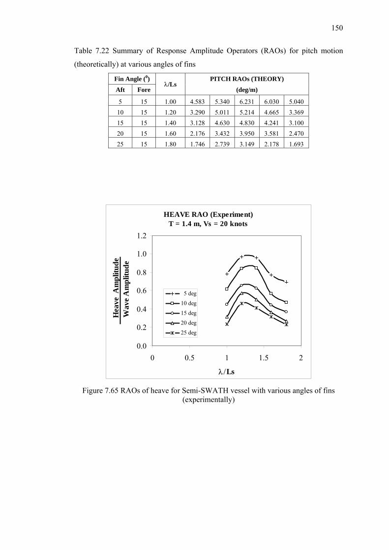
150
Table 7.22 Summary of Response Amplitude Operators (RAOs) for pitch motion
(theoretically) at various angles of fins
Fin Angle (0) PITCH RAOs (THEORY)
Aft Fore λ/Ls
(deg/m)
5 15 1.00 4.583 5.340 6.231 6.030 5.040 10 15 1.20 3.290 5.011 5.214 4.665 3.369 15 15 1.40 3.128 4.630 4.830 4.241 3.100 20 15 1.60 2.176 3.432 3.950 3.581 2.470 25 15 1.80 1.746 2.739 3.149 2.178 1.693
HEAVE RAO (Experiment)T = 1.4 m, Vs = 20 knots
0.0
0.2
0.4
0.6
0.8
1.0
1.2
0 0.5 1 1.5 2
λ/Ls
H
eave
Am
plitu
de
Wav
e A
mpl
itude
5 deg
10 deg
15 deg
20 deg
25 deg
Figure 7.65 RAOs of heave for Semi-SWATH vessel with various angles of fins
(experimentally)
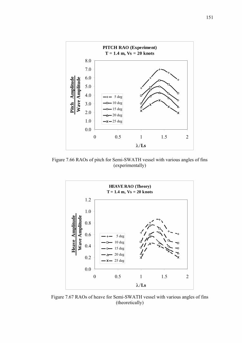
151
PITCH RAO (Experiment)T = 1.4 m, Vs = 20 knots
0.0
1.0
2.0
3.0
4.0
5.0
6.0
7.0
8.0
0 0.5 1 1.5 2
λ/Ls
Pitc
h A
mpl
itude
W
ave
Am
plitu
de
5 deg
10 deg
15 deg
20 deg
25 deg
Figure 7.66 RAOs of pitch for Semi-SWATH vessel with various angles of fins (experimentally)
HEAVE RAO (Theory)T = 1.4 m, Vs = 20 knots
0.0
0.2
0.4
0.6
0.8
1.0
1.2
0 0.5 1 1.5 2
λ/Ls
Hea
ve A
mpl
itude
W
ave
Am
plitu
de
5 deg
10 deg
15 deg
20 deg
25 deg
Figure 7.67 RAOs of heave for Semi-SWATH vessel with various angles of fins
(theoretically)
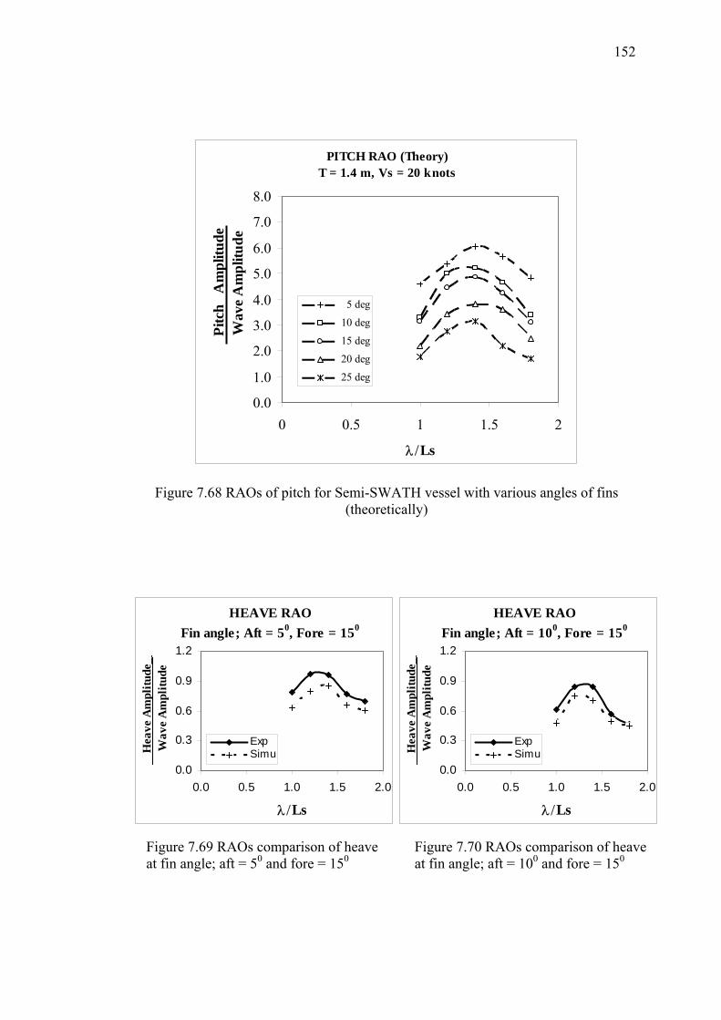
152
PITCH RAO (Theory)T = 1.4 m, Vs = 20 knots
0.0
1.0
2.0
3.0
4.0
5.0
6.0
7.0
8.0
0 0.5 1 1.5 2
λ/Ls
Pitc
h A
mpl
itude
W
ave
Am
plitu
de
5 deg
10 deg
15 deg
20 deg
25 deg
Figure 7.68 RAOs of pitch for Semi-SWATH vessel with various angles of fins (theoretically)
Figure 7.69 RAOs comparison of heaveat fin angle; aft = 50 and fore = 150
Figure 7.70 RAOs comparison of heaveat fin angle; aft = 100 and fore = 150
HEAVE RAOFin angle; Aft = 50, Fore = 150
0.0
0.3
0.6
0.9
1.2
0.0 0.5 1.0 1.5 2.0
λ/Ls
H
eave
Am
plitu
de__
Wav
e A
mpl
itude
ExpSimu
HEAVE RAOFin angle; Aft = 100, Fore = 150
0.0
0.3
0.6
0.9
1.2
0.0 0.5 1.0 1.5 2.0
λ/Ls
H
eave
Am
plitu
de__
Wav
e A
mpl
itude
ExpSimu
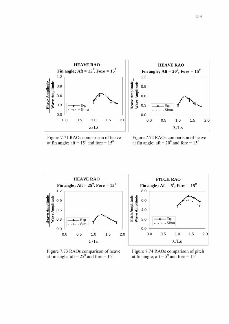
153
Figure 7.71 RAOs comparison of heaveat fin angle; aft = 150 and fore = 150
Figure 7.72 RAOs comparison of heaveat fin angle; aft = 200 and fore = 150
HEAVE RAOFin angle; Aft = 150, Fore = 150
0.0
0.3
0.6
0.9
1.2
0.0 0.5 1.0 1.5 2.0
λ/Ls
H
eave
Am
plitu
de__
Wav
e A
mpl
itude
ExpSimu
HEAVE RAOFin angle; Aft = 200, Fore = 150
0.0
0.3
0.6
0.9
1.2
0.0 0.5 1.0 1.5 2.0
λ/Ls
Hea
ve A
mpl
itude
__W
ave
Am
plitu
de
ExpSimu
Figure 7.73 RAOs comparison of heaveat fin angle; aft = 250 and fore = 150
Figure 7.74 RAOs comparison of pitch at fin angle; aft = 50 and fore = 150
PITCH RAOFin angle; Aft = 50, Fore = 150
0.0
2.0
4.0
6.0
8.0
0.0 0.5 1.0 1.5 2.0
λ/Ls
P
itch
Am
plitu
de_
Wav
e A
mpl
itude
ExpSimu
HEAVE RAOFin angle; Aft = 250, Fore = 150
0.0
0.3
0.6
0.9
1.2
0.0 0.5 1.0 1.5 2.0
λ/Ls
H
eave
Am
plitu
de__
Wav
e A
mpl
itude
ExpSimu
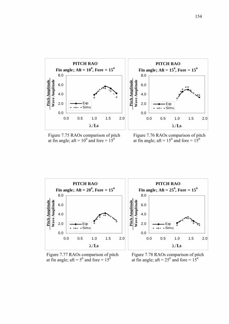
154
Figure 7.77 RAOs comparison of pitch at fin angle; aft = 50 and fore = 150
Figure 7.78 RAOs comparison of pitch at fin angle; aft = 250 and fore = 150
PITCH RAOFin angle; Aft = 200, Fore = 150
0.0
2.0
4.0
6.0
8.0
0.0 0.5 1.0 1.5 2.0
λ/Ls
P
itch
Am
plitu
de_
Wav
e A
mpl
itude
ExpSimu
PITCH RAOFin angle; Aft = 250, Fore = 150
0.0
2.0
4.0
6.0
8.0
0.0 0.5 1.0 1.5 2.0
λ/Ls
P
itch
Am
plitu
de_
Wav
e A
mpl
itude
ExpSimu
Figure 7.75 RAOs comparison of pitch at fin angle; aft = 100 and fore = 150
Figure 7.76 RAOs comparison of pitch at fin angle; aft = 150 and fore = 150
PITCH RAOFin angle; Aft = 150, Fore = 150
0.0
2.0
4.0
6.0
8.0
0.0 0.5 1.0 1.5 2.0
λ/Ls
Pitc
h A
mpl
itude
_W
ave
Am
plitu
de
ExpSimu
PITCH RAOFin angle; Aft = 100, Fore = 150
0.0
2.0
4.0
6.0
8.0
0.0 0.5 1.0 1.5 2.0
λ/Ls
P
itch
Am
plitu
de_
Wav
e A
mpl
itude
ExpSimu
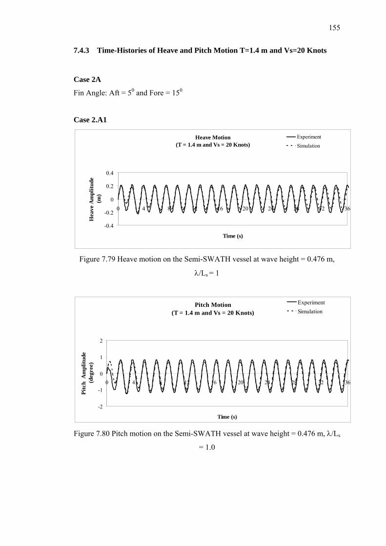
155
7.4.3 Time-Histories of Heave and Pitch Motion T=1.4 m and Vs=20 Knots
Case 2A
Fin Angle: Aft = 50 and Fore = 150
Case 2.A1
Heave Motion(T = 1.4 m and Vs = 20 Knots)
-0.4
-0.2
0
0.2
0.4
0 4 8 12 16 20 24 28 32 36
Time (s)
Hea
ve A
mpl
itude
(m
)
Experiment
Simulation
Figure 7.79 Heave motion on the Semi-SWATH vessel at wave height = 0.476 m,
λ/Ls = 1
Pitch Motion(T = 1.4 m and Vs = 20 Knots)
-2
-1
0
1
2
0 4 8 12 16 20 24 28 32 36
Time (s)
Pitc
h A
mpl
itude
(d
egre
e)
ExperimentSimulation
Figure 7.80 Pitch motion on the Semi-SWATH vessel at wave height = 0.476 m, λ/Ls
= 1.0
156
Case 2.A2
Heave Motion(T = 1.4 m and Vs = 20 Knots)
-0.4
-0.2
0
0.2
0.4
0 4 8 12 16 20 24 28 32 36
Time (s)
Hea
ve A
mpl
itude
(m
)
ExperimentSimulation
Figure 7.81 Heave motion on the Semi-SWATH vessel at wave height = 0.571 m,
λ/Ls = 1.2
Pitch Motion(T = 1.4 m and Vs = 20 Knots)
-3
-1.5
0
1.5
3
0 4 8 12 16 20 24 28 32 36
Time (s)
Pitc
h A
mpl
itude
(d
egre
e)
ExperimentSimulation
Figure 7.82 Pitch motion on the Semi-SWATH vessel at wave height = 0.571 m, λ/Ls
= 1.2
157
Case 2.A3
Heave Motion(T = 1.4 m and Vs = 20 Knots)
-0.4
-0.2
0
0.2
0.4
0 4 8 12 16 20 24 28 32 36
Time (s)
Hea
ve A
mpl
itude
(m)
ExperimentSimulation
Figure 7.83 Heave motion on the Semi-SWATH vessel at wave height = 0.666 m,
λ/Ls = 1.4
Pitch Motion(T = 1.4 m and Vs = 20 Knots)
-4-3-2-10123
0 4 8 12 16 20 24 28 32 36
Time (s)
Pitc
h A
mpl
itude
(d
egre
e)
ExperimentSimulation
Figure 7.84 Pitch motion on the Semi-SWATH vessel at wave height = 0.666 m, λ/Ls
= 1.4
158
Case 2.A4
Heave Motion(T = 1.4 m and Vs = 20 Knots)
-0.4
-0.2
0
0.2
0.4
0 4 8 12 16 20 24 28 32 36 40
Time (s)
Hea
ve A
mpl
itude
(m)
ExperimentSimulation
Figure 7.85 Heave motion on the Semi-SWATH vessel at wave height = 0.762 m,
λ/Ls = 1.6
Pitch Motion(T = 1.4 m and Vs = 20 Knots)
-4
-2
0
2
4
0 4 8 12 16 20 24 28 32 36 40
Time (s)
Pitc
h A
mpl
itude
(d
egre
e)
ExperimentSimulation
Figure 7.86 Pitch motion on the Semi-SWATH vessel at wave height = 0.762 m, λ/Ls
= 1.6
159
Case 2.A5
Heave Motion(T = 1.4 m and Vs = 20 Knots)
-0.4
-0.2
0
0.2
0.4
0 4 8 12 16 20 24 28 32 36 40
Time (s)
Hea
ve A
mpl
itude
(m
)
Experiment
Simulation
Figure 7.87 Heave motion on the Semi-SWATH vessel at wave height = 0.857 m,
λ/Ls = 1.8
Pitch Motion(T = 1.4 m and Vs = 20 Knots)
-4
-2
0
2
4
0 4 8 12 16 20 24 28 32 36
Time (s)
Pitc
h A
mpl
itude
(d
egre
e)
ExperimentSimulation
Figure 7.88 Pitch motion on the Semi-SWATH vessel at wave height = 0.857 m, λ/Ls
= 1.8
160
Case 2B
Fin Angle: Aft =100 and Fore = 150
Case 2.B1
Heave Motion(T = 1.4 m and Vs = 20 Knots)
-0.3
-0.2-0.1
00.1
0.20.3
0 4 8 12 16 20 24 28 32 36 40
Time (s)
Hea
ve A
mpl
itude
(m)
ExperimentSimulation
Figure 7.89 Heave motion on the Semi-SWATH vessel at wave height = 0.476 m,
λ/Ls = 1.0
Pitch Motion(T = 1.4 m and Vs = 20 Knots)
-2
-1
0
1
2
0 4 8 12 16 20 24 28 32 36 40 44
Time (s)
Pitc
h A
mpl
itude
(d
egre
e)
ExperimentSimulation
Figure 7.90 Pitch motion on the Semi-SWATH vessel at wave height = 0.476 m,
λ/Ls = 1.0
161
Case 2.B2
Heave Motion(T = 1.4 m and Vs = 20 Knots)
-0.3-0.2-0.1
00.10.20.30.40.5
0 4 8 12 16 20 24 28 32 36 40 44
Time (s)
Hea
ve A
mpl
itude
(m)
ExperimentSimulation
Figure 7.91 Heave motion on the Semi-SWATH vessel at wave height = 0.571 m,
λ/Ls = 1.2
Pitch Motion(T = 1.4 m and Vs = 20 Knots)
-3
-2
-1
0
1
2
3
0 4 8 12 16 20 24 28 32 36 40
Time (s)
Pitc
h A
mpl
itude
(d
egre
e)
ExperimentSimulation
Figure 7.92 Pitch motion on the Semi-SWATH vessel at wave height = 0.571 m, λ/Ls
= 1.2
162
Case 2.B3
Heave Motion(T = 1.4 m and Vs = 20 Knots)
-0.3-0.2-0.1
00.10.20.30.4
0 4 8 12 16 20 24 28 32 36
Time (s)
Hea
ve A
mpl
itude
(m)
ExperimentSimulation
Figure 7.93 Heave motion on the Semi-SWATH vessel at wave height = 0.666 m,
λ/Ls = 1.4
Pitch Motion(T = 1.4 m and Vs = 20 Knots)
-4
-3
-2
-1
0
1
2
3
0 4 8 12 16 20 24 28 32 36 40
Time (s)
Pitc
h A
mpl
itude
(d
egre
e)
ExperimentSimulation
Figure 7.94 Pitch motion on the Semi-SWATH vessel at wave height = 0.666 m, λ/Ls
= 1.4
163
Case 2.B4
Heave Motion(T = 1.4 m and Vs = 20 Knots)
-0.4
-0.2
0
0.2
0.4
0 4 8 12 16 20 24 28 32 36
Time (s)
Hea
ve A
mpl
itude
(m)
ExperimentSimulation
Figure 7.95 Heave motion on the Semi-SWATH vessel at wave height = 0.762 m,
λ/Ls = 1.6
Pitch Motion(T = 1.4 m and Vs = 20 Knots)
-4
-2
0
2
4
0 4 8 12 16 20 24 28 32 36
Time (s)
Pitc
h A
mpl
itude
(d
egre
e)
ExperimentSimulation
Figure 7.96 Pitch motion on the Semi-SWATH vessel at wave height = 0.762 m, λ/Ls
= 1.6
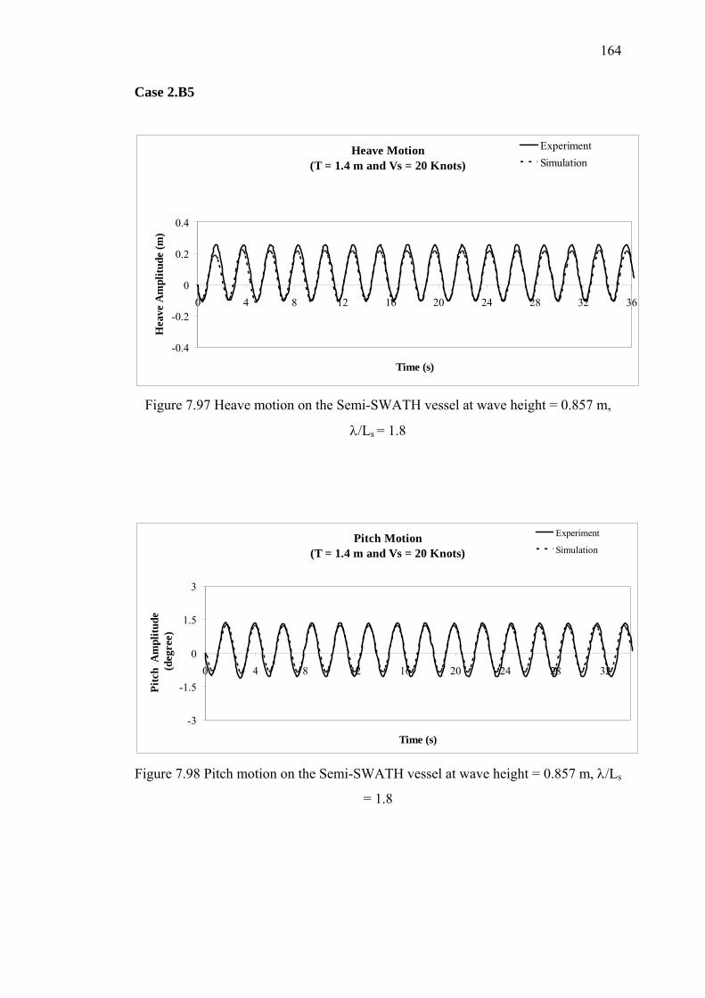
164
Case 2.B5
Heave Motion(T = 1.4 m and Vs = 20 Knots)
-0.4
-0.2
0
0.2
0.4
0 4 8 12 16 20 24 28 32 36
Time (s)
Hea
ve A
mpl
itude
(m)
ExperimentSimulation
Figure 7.97 Heave motion on the Semi-SWATH vessel at wave height = 0.857 m,
λ/Ls = 1.8
Pitch Motion(T = 1.4 m and Vs = 20 Knots)
-3
-1.5
0
1.5
3
0 4 8 12 16 20 24 28 32
Time (s)
Pitc
h A
mpl
itude
(d
egre
e)
Experiment
Simulation
Figure 7.98 Pitch motion on the Semi-SWATH vessel at wave height = 0.857 m, λ/Ls
= 1.8
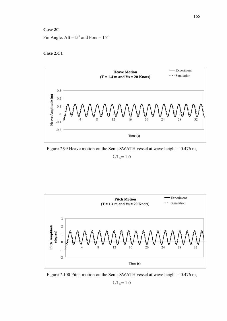
165
Case 2C
Fin Angle: Aft =150 and Fore = 150
Case 2.C1
Heave Motion(T = 1.4 m and Vs = 20 Knots)
-0.2
-0.1
0
0.1
0.2
0.3
0 4 8 12 16 20 24 28 32
Time (s)
Hea
ve A
mpl
itude
(m)
ExperimentSimulation
Figure 7.99 Heave motion on the Semi-SWATH vessel at wave height = 0.476 m,
λ/Ls = 1.0
Pitch Motion(T = 1.4 m and Vs = 20 Knots)
-2
-1
0
1
2
3
0 4 8 12 16 20 24 28 32
Time (s)
Pitc
h A
mpl
itude
(d
egre
e)
ExperimentSimulation
Figure 7.100 Pitch motion on the Semi-SWATH vessel at wave height = 0.476 m,
λ/Ls = 1.0
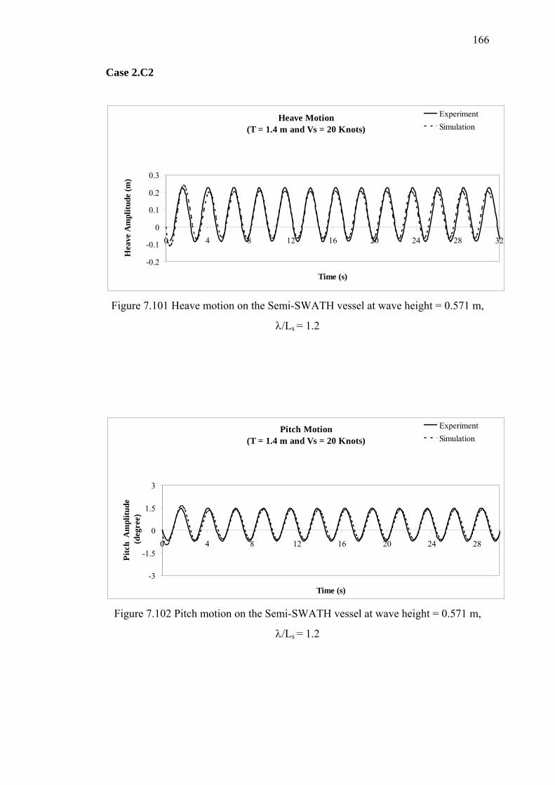
166
Case 2.C2
Heave Motion(T = 1.4 m and Vs = 20 Knots)
-0.2
-0.1
0
0.1
0.2
0.3
0 4 8 12 16 20 24 28 32
Time (s)
Hea
ve A
mpl
itude
(m)
ExperimentSimulation
Figure 7.101 Heave motion on the Semi-SWATH vessel at wave height = 0.571 m,
λ/Ls = 1.2
Pitch Motion(T = 1.4 m and Vs = 20 Knots)
-3
-1.5
0
1.5
3
0 4 8 12 16 20 24 28
Time (s)
Pitc
h A
mpl
itude
(d
egre
e)
ExperimentSimulation
Figure 7.102 Pitch motion on the Semi-SWATH vessel at wave height = 0.571 m,
λ/Ls = 1.2
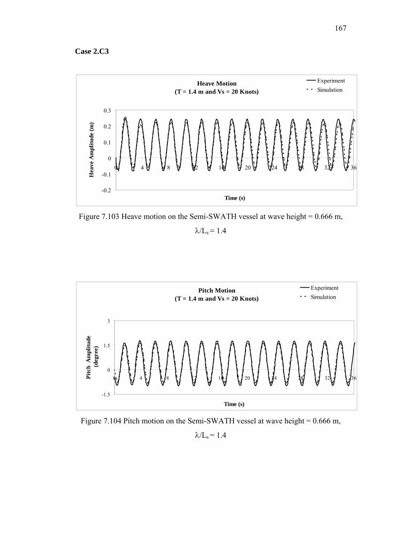
167
Case 2.C3
Heave Motion(T = 1.4 m and Vs = 20 Knots)
-0.2
-0.1
0
0.1
0.2
0.3
0 4 8 12 16 20 24 28 32 36
Time (s)
Hea
ve A
mpl
itude
(m)
ExperimentSimulation
Figure 7.103 Heave motion on the Semi-SWATH vessel at wave height = 0.666 m,
λ/Ls = 1.4
Pitch Motion(T = 1.4 m and Vs = 20 Knots)
-1.5
0
1.5
3
0 4 8 12 16 20 24 28 32 36
Time (s)
Pitc
h A
mpl
itude
(d
egre
e)
ExperimentSimulation
Figure 7.104 Pitch motion on the Semi-SWATH vessel at wave height = 0.666 m,
λ/Ls = 1.4
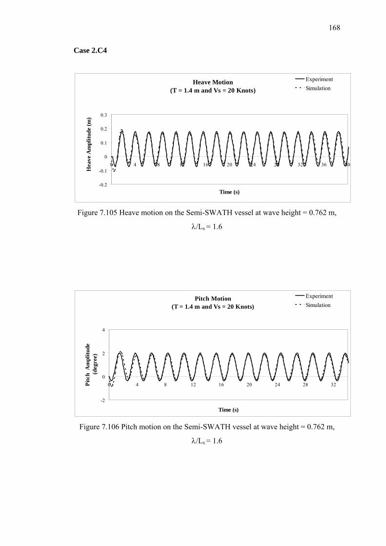
168
Case 2.C4
Heave Motion(T = 1.4 m and Vs = 20 Knots)
-0.2
-0.1
0
0.1
0.2
0.3
0 4 8 12 16 20 24 28 32 36 40
Time (s)
Hea
ve A
mpl
itude
(m)
ExperimentSimulation
Figure 7.105 Heave motion on the Semi-SWATH vessel at wave height = 0.762 m,
λ/Ls = 1.6
Pitch Motion(T = 1.4 m and Vs = 20 Knots)
-2
0
2
4
0 4 8 12 16 20 24 28 32
Time (s)
Pitc
h A
mpl
itude
(d
egre
e)
ExperimentSimulation
Figure 7.106 Pitch motion on the Semi-SWATH vessel at wave height = 0.762 m,
λ/Ls = 1.6
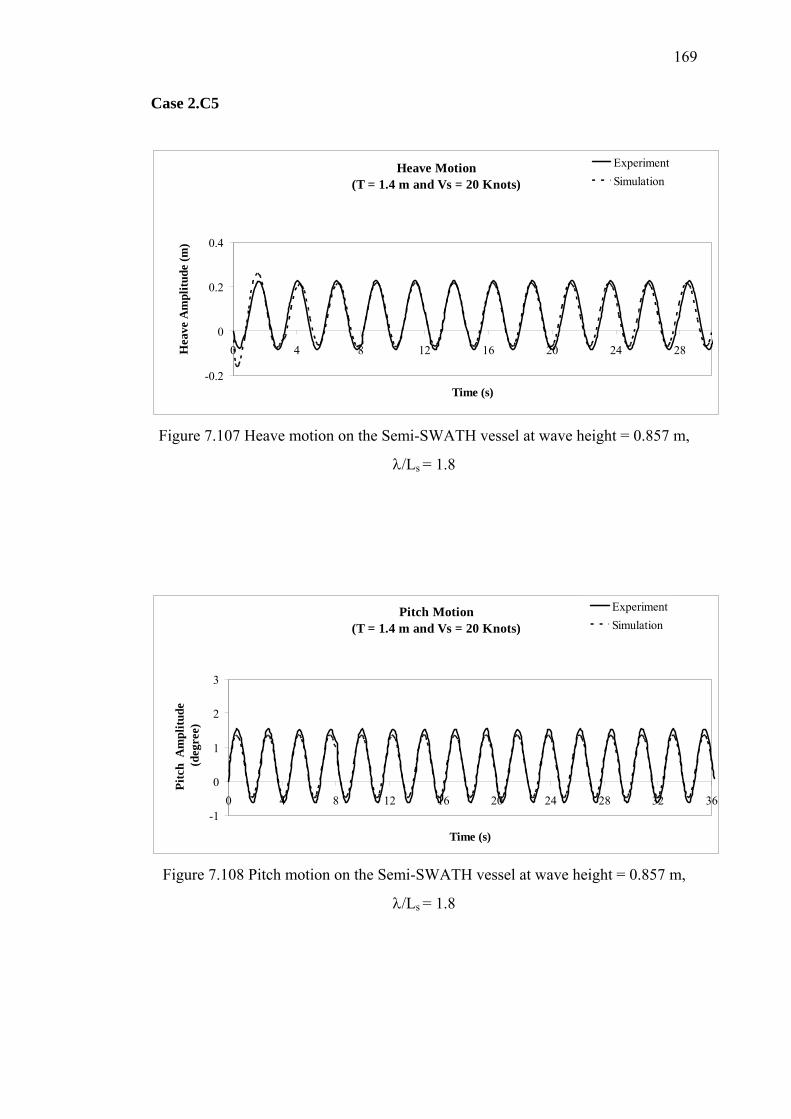
169
Case 2.C5
Heave Motion(T = 1.4 m and Vs = 20 Knots)
-0.2
0
0.2
0.4
0 4 8 12 16 20 24 28
Time (s)
Hea
ve A
mpl
itude
(m)
ExperimentSimulation
Figure 7.107 Heave motion on the Semi-SWATH vessel at wave height = 0.857 m,
λ/Ls = 1.8
Pitch Motion(T = 1.4 m and Vs = 20 Knots)
-1
0
1
2
3
0 4 8 12 16 20 24 28 32 36
Time (s)
Pitc
h A
mpl
itude
(d
egre
e)
ExperimentSimulation
Figure 7.108 Pitch motion on the Semi-SWATH vessel at wave height = 0.857 m,
λ/Ls = 1.8
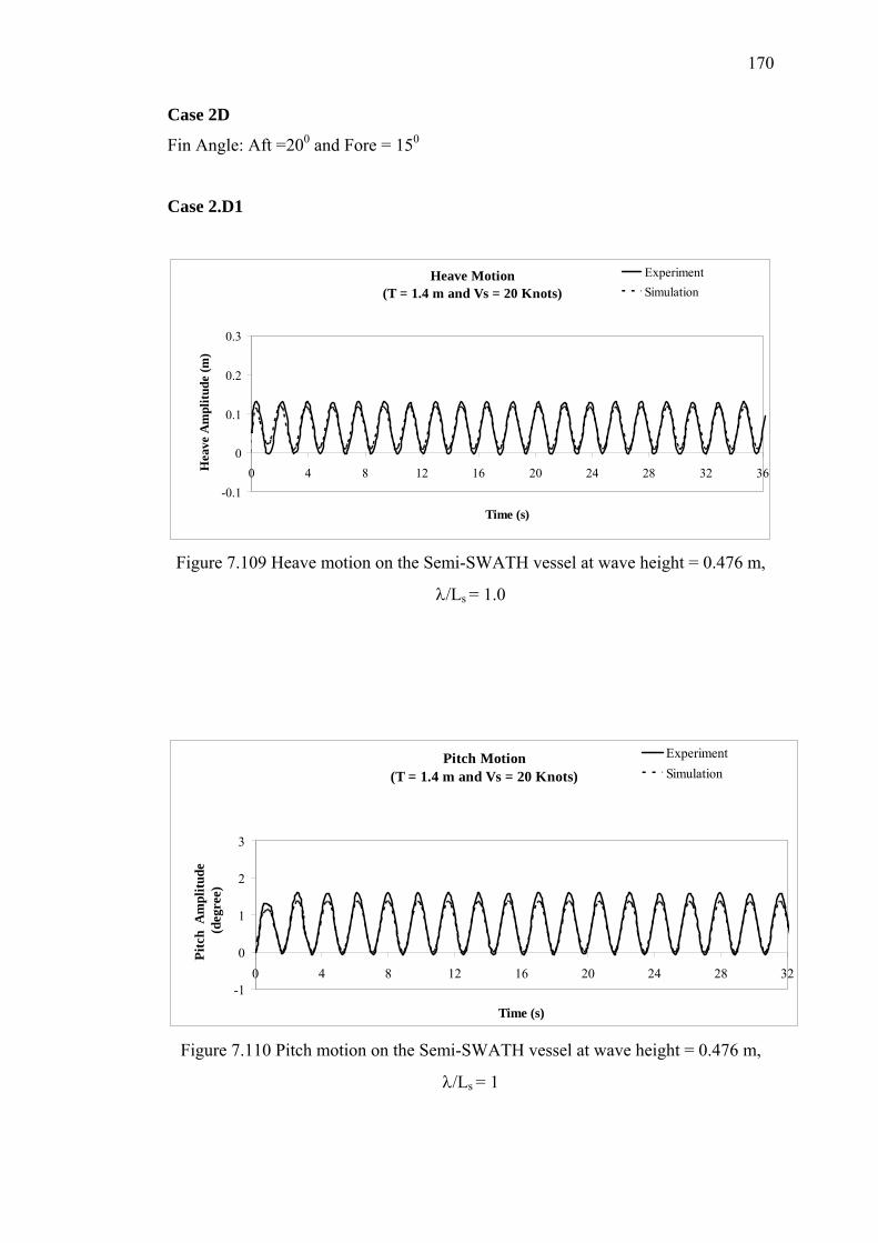
170
Case 2D
Fin Angle: Aft =200 and Fore = 150
Case 2.D1
Heave Motion(T = 1.4 m and Vs = 20 Knots)
-0.1
0
0.1
0.2
0.3
0 4 8 12 16 20 24 28 32 36
Time (s)
Hea
ve A
mpl
itude
(m)
ExperimentSimulation
Figure 7.109 Heave motion on the Semi-SWATH vessel at wave height = 0.476 m,
λ/Ls = 1.0
Pitch Motion(T = 1.4 m and Vs = 20 Knots)
-1
0
1
2
3
0 4 8 12 16 20 24 28 32
Time (s)
Pitc
h A
mpl
itude
(d
egre
e)
ExperimentSimulation
Figure 7.110 Pitch motion on the Semi-SWATH vessel at wave height = 0.476 m,
λ/Ls = 1
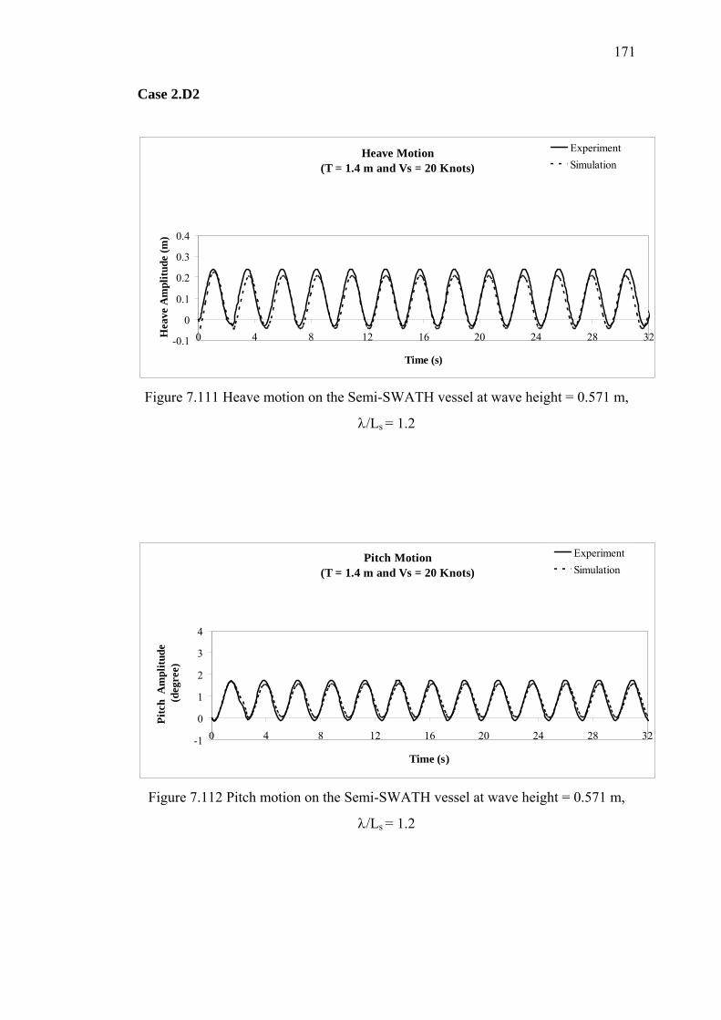
171
Case 2.D2
Heave Motion(T = 1.4 m and Vs = 20 Knots)
-0.1
0
0.1
0.2
0.3
0.4
0 4 8 12 16 20 24 28 32
Time (s)
Hea
ve A
mpl
itude
(m)
ExperimentSimulation
Figure 7.111 Heave motion on the Semi-SWATH vessel at wave height = 0.571 m,
λ/Ls = 1.2
Pitch Motion(T = 1.4 m and Vs = 20 Knots)
-1
0
1
2
3
4
0 4 8 12 16 20 24 28 32
Time (s)
Pitc
h A
mpl
itude
(d
egre
e)
ExperimentSimulation
Figure 7.112 Pitch motion on the Semi-SWATH vessel at wave height = 0.571 m,
λ/Ls = 1.2
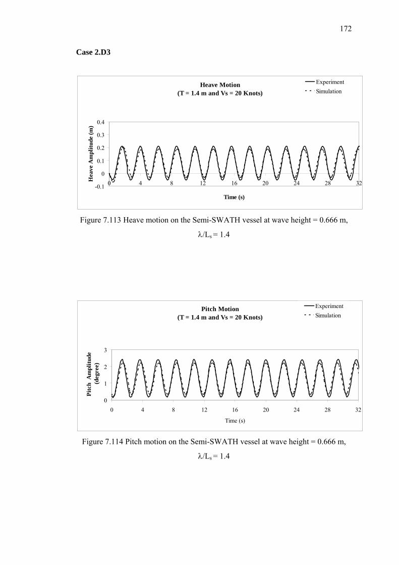
172
Case 2.D3
Heave Motion(T = 1.4 m and Vs = 20 Knots)
-0.1
0
0.1
0.2
0.3
0.4
0 4 8 12 16 20 24 28 32
Time (s)
Hea
ve A
mpl
itude
(m)
ExperimentSimulation
Figure 7.113 Heave motion on the Semi-SWATH vessel at wave height = 0.666 m,
λ/Ls = 1.4
Pitch Motion(T = 1.4 m and Vs = 20 Knots)
0
1
2
3
0 4 8 12 16 20 24 28 32
Time (s)
Pitc
h A
mpl
itude
(d
egre
e)
ExperimentSimulation
Figure 7.114 Pitch motion on the Semi-SWATH vessel at wave height = 0.666 m,
λ/Ls = 1.4
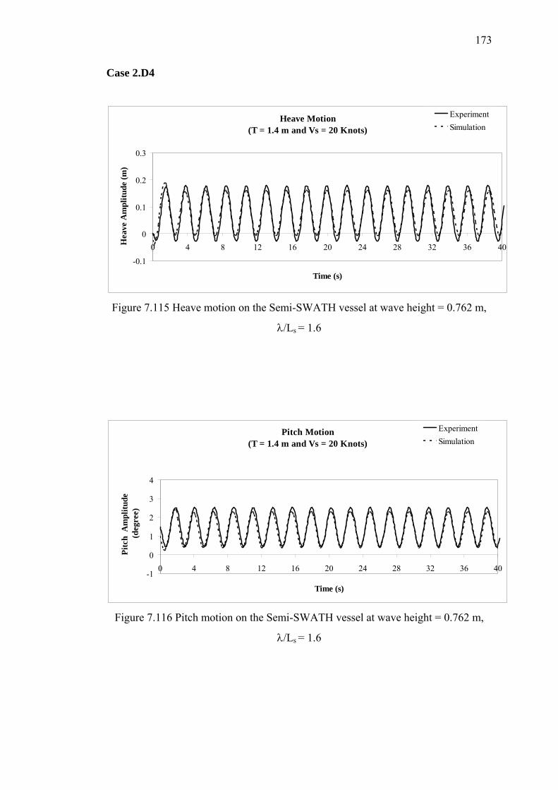
173
Case 2.D4
Heave Motion(T = 1.4 m and Vs = 20 Knots)
-0.1
0
0.1
0.2
0.3
0 4 8 12 16 20 24 28 32 36 40
Time (s)
Hea
ve A
mpl
itude
(m)
ExperimentSimulation
Figure 7.115 Heave motion on the Semi-SWATH vessel at wave height = 0.762 m,
λ/Ls = 1.6
Pitch Motion(T = 1.4 m and Vs = 20 Knots)
-1
0
1
2
3
4
0 4 8 12 16 20 24 28 32 36 40
Time (s)
Pitc
h A
mpl
itude
(d
egre
e)
ExperimentSimulation
Figure 7.116 Pitch motion on the Semi-SWATH vessel at wave height = 0.762 m,
λ/Ls = 1.6
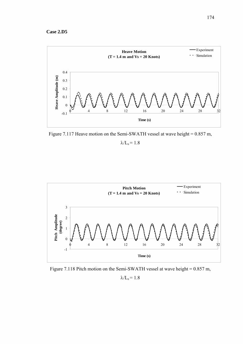
174
Case 2.D5
Heave Motion(T = 1.4 m and Vs = 20 Knots)
-0.1
0
0.1
0.2
0.3
0.4
0 4 8 12 16 20 24 28 32
Time (s)
Hea
ve A
mpl
itude
(m)
ExperimentSimulation
Figure 7.117 Heave motion on the Semi-SWATH vessel at wave height = 0.857 m,
λ/Ls = 1.8
Pitch Motion(T = 1.4 m and Vs = 20 Knots)
-1
0
1
2
3
0 4 8 12 16 20 24 28 32
Time (s)
Pitc
h A
mpl
itude
(d
egre
e)
ExperimentSimulation
Figure 7.118 Pitch motion on the Semi-SWATH vessel at wave height = 0.857 m,
λ/Ls = 1.8
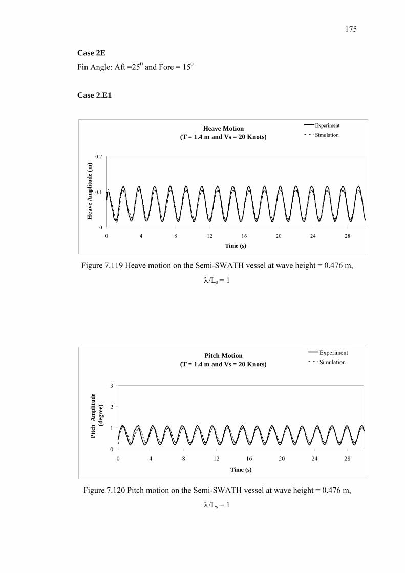
175
Case 2E
Fin Angle: Aft =250 and Fore = 150
Case 2.E1
Heave Motion(T = 1.4 m and Vs = 20 Knots)
0
0.1
0.2
0 4 8 12 16 20 24 28
Time (s)
Hea
ve A
mpl
itude
(m)
Experiment
Simulation
Figure 7.119 Heave motion on the Semi-SWATH vessel at wave height = 0.476 m,
λ/Ls = 1
Pitch Motion(T = 1.4 m and Vs = 20 Knots)
0
1
2
3
0 4 8 12 16 20 24 28
Time (s)
Pitc
h A
mpl
itude
(d
egre
e)
ExperimentSimulation
Figure 7.120 Pitch motion on the Semi-SWATH vessel at wave height = 0.476 m,
λ/Ls = 1
176
Case 2.E2
Heave Motion(T = 1.4 m and Vs = 20 Knots)
-0.1
0
0.1
0.2
0.3
0 4 8 12 16 20 24 28 32 36 40
Time (s)
Hea
ve A
mpl
itude
(m)
ExperimentSimulation
Figure 7.121 Heave motion on the Semi-SWATH vessel at wave height = 0.571 m,
λ/Ls = 1.2
Pitch Motion(T = 1.4 m and Vs = 20 Knots)
0
1
2
3
4
0 4 8 12 16 20 24 28 32
Time (s)
Pitc
h A
mpl
itude
(d
egre
e)
ExperimentSimulation
Figure 7.122 Pitch motion on the Semi-SWATH vessel at wave height = 0.571 m,
λ/Ls = 1.2
177
Case 2.E3
Heave Motion(T = 1.4 m and Vs = 20 Knots)
-0.1
0
0.1
0.2
0.3
0.4
0 4 8 12 16 20 24 28 32 36
Time (s)
Hea
ve A
mpl
itude
(m)
ExperimentSimulation
Figure 7.123 Heave motion on the Semi-SWATH vessel at wave height = 0.666 m,
λ/Ls = 1.4
Pitch Motion(T = 1.4 m and Vs = 20 Knots)
-1
0
1
2
3
4
0 4 8 12 16 20 24 28 32
Time (s)
Pitc
h A
mpl
itude
(d
egre
e)
ExperimentSimulation
Figure 7.124 Pitch motion on the Semi-SWATH vessel at wave height = 0.666 m,
λ/Ls = 1.4
178
Case 2.E4
Heave Motion(T = 1.4 m and Vs = 20 Knots)
-0.1
0
0.1
0.2
0.3
0.4
0 4 8 12 16 20 24 28
Time (s)
Hea
ve A
mpl
itude
(m)
ExperimentSimulation
Figure 7.125 Heave motion on the Semi-SWATH vessel at wave height = 0.762 m,
λ/Ls = 1.6
Pitch Motion(T = 1.4 m and Vs = 20 Knots)
-1
0
1
2
3
0 4 8 12 16 20 24 28
Time (s)
Pitc
h A
mpl
itude
(d
egre
e)
ExperimentSimulation
Figure 7.126 Pitch motion on the Semi-SWATH vessel at wave height = 0.762 m,
λ/Ls = 1.6
179
Case 2.E5
Heave Motion(T = 1.4 m and Vs = 20 Knots)
-0.1
0
0.1
0.2
0.3
0.4
0 4 8 12 16 20 24 28 32
Time (s)
Hea
ve A
mpl
itude
(m)
ExperimentSimulation
Figure 7.127 Heave motion on the Semi-SWATH vessel at wave height = 0.857 m,
λ/Ls = 1.8
Pitch Motion(T = 1.4 m and Vs = 20 Knots)
-1
0
1
2
3
0 4 8 12 16 20 24 28
Time (s)
Pitc
h A
mpl
itude
(d
egre
e)
ExperimentSimulation
Figure 7.128 Pitch motion on the Semi-SWATH vessel at wave height = 0.857 m,
λ/Ls = 1.8

180
7.5 Concluding Remarks
Generally, the comparison between simulation program and experimental
results, gives confidence to develop seakeeping prediction by utilising the simulation
program. Qualitatively, the present mathematical model successfully simulate the
motion response prediction of heave and pitch for a Semi-SWATH vessel both with
and without fin stabilizers at medium (15 knots) and high-speed (20 knots)
conditions at range ratio of wavelengths to the model length (Ship
λL
) is about 0.5-2.5
with wave height to wavelength ratio at the experiments was 1/25.
CHAPTER 8
DISCUSSION
8.1 General
The twin-hull vessels are known to have more stable platform and provides a
better seakeeping qualities as compared to mono-hull. However, the significant
drawback of the twin-hull vessel especially Semi-SWATH vessel is when
encountering head-sea at high forward speed. Due to its low stiffness, it has a
tendency for large pitch motions. In this condition, deck wetness, slamming, and
structural damage are the most dangerous situation that should be considered in
vessel seakeeping performances. For this reason, two modes of coupled motions are
considered in this study, there are heave and pitch motions as the main parametric
that have quite contributions affected to seakeeping qulity of Semi-SWATH vessel.
Since the non-linear mode both of heave and pitching responses are
considered, Time Domain Simulation approach is utilized to solve the equations of
motion. One of the important aspects of the present simulation program is the
calculation and evaluation of seakeeping performance in step of time inherent to the
bare hull vessel and after present an additional damping due to two pairs of fin
stabilizers on the Semi-SWATH hull in waves.
A simulation procedure had been followed to conduct parameter study in
systematic way. The main purpose of the parametric study is to compare motion
characteristics of different conditions i.e. bare hull condition and after installed fixed
182
and controllable fin stabilizers at two operational draughts (shallow water and deep
water) with different service speeds i.e. 15 knots (medium speed) and 20 knots (high-
speed) by utilizing the Time Domain Simulation approach.
In case on the simulation of controllable aft fin stabilizers, the conventional
PID controller will be applied to refine the plant system. For that reason, the vessel
will experience a better ride performance with more improvement of reduction of
heave and pitch motion compared to uncontrolled fin. In addition, the simulation and
experiments results obtained through the parametric study become a guideline
prediction of vessels’ comfortability. Simply, the study of the seakeeping evaluation
of Semi-SWATH vessel was divided into four sections, as follow;
1. The first involved the development of the mathematical model for
simulation purposes. The fin angles with fixed and controllable fin
inclined relative to the main hull body have to be adequate to have a
significant effect on the seakeeping performance of Semi-SWATH
vessel during sailing.
2. The second investigate of the controller scheme of the controllable aft
fin stabilizer on the vessel performances.
3. The third involved the development of PID controller that applied on
the controllable aft fins to obtain a better ride performance of Semi-
SWATH vessel passengers comfort, which give a more significant
reduction of heave and pitch motions than using fixed fins.
4. The fourth, the experimental work of seakeeping study will be
conducted to validate the derived mathematical model that has been
conducted in PC base simulation program. In this case, the validation
is only to justify the simulation condition on bare hull vessel and
using fixed fin relative to the main hull body only.
183
8.2 Mathematical model
In the present study, the main interest is given on the ship motion in head seas
condition. Basically, the modular mathematical model has been chosen for this study.
The motion system of the vessel consists two-degrees-of-freedom i.e. coupled heave
and pitch motions. The mathematical model comprising of heave and pitch motions,
which incorporated with fixed and controllable fins stabilizers on the simulation was
presented in a simple block diagram using Matlab-SIMULINK.
A computation procedure to calculate the forces up to free surface has been
applied to obtain the hydrostatic forces including restoring forces and Froude-Krylov
forces and lift forces due to fin stabilizers. This computation procedure successfully
simulates heave and pitch motion responses both of bare vessel and after attached
fixed and controllable fins.
For the hydrodynamic forces, it is determined through the empirical
formulations. However, the mathematical model requires coefficients such as added
mass and damping and restoring moment. These coefficients are obtained directly
through the published literature or experiment. Frank-Close Fit method (Atlar, 1982)
and Maimun (1993) experimental results are the two important references to estimate
the coefficients. This study showed that ship motion is sensitive to the change of
pitch restoring. Therefore, pitch restoring force should be accurately determined in
thesimulation run.
8.3 Investigation of Controller Scheme of The Fin Stabilizers
In this investigation, the controller scheme of fin stabilizer was applied
into two rules, namely;
a) Fin with constant inclined angle relative the main hull body
This case means that the stabilizer fin is adjusted to have an inclined
angle relative to the ship body. The total lift on the ship is then due to the
resultant of angle of attack of incident flow to the body and the inclined
184
angle of fin. This technique can be applied to adjust the trim condition of
Semi-SWATH vessel advancing in waves with initial trim by bow or
stern.
In this work, the aft and fore fin with fixed angle inclined relative to the
main hull body. This case is achieved by adjusting manually the
stabilizer fin to be with a constant angle of fins relative to the main hull
body while the Semi-SWATH vessel running in waves. The gradual
adjustable angle of the aft fin will result the heave and pitch motion
decreases equals to their positive inclined angles of fixed fore fin (150)
and fixed aft fin of 50, 100, 150, 200, and 250 relative to the main hull. The
maximum reduction of heave and pitch motion are about 40.14% and
37.95% (Figure 7.35 and Figure 7.44).
b) Time-Varying Controllable Fin
The purpose of this technique is to obtain more improvement of reducing
heave and pitch motions of the Semi-SWATH vessel advancing in waves.
The principle is to adjust the fin lift force to balance the force due wave
excitation on the Semi-SWATH vessel.
In this work, by controlling the aft fins properly, the sailing style of Semi-
SWATH vessel may be more effective than uncontrolled one. The aft
fins control (δaft) were set by 00 up to 250 and fixed fore fins (δfore) is set
by 150. The aft fins are controlled which the all fixed operated fins angle
speeds of 22.50/sec. We find that the quick operated speed affects the
pitch motion faster reduced. This control scheme is quite reasonable
because the system response is more stable. In this case, the controllable
aft fins can be operated more secure and smoothly and a gradual response
is achieved too. Practically, the aft fins are controlled simultaneously to
achieve a better operation condition.
185
8.4 Development of PID Controller
The present study concentrates on the solution of ship motion reduction
especially for heave and pitch motions in head-seas condition due to controllable aft
fin stabilizers. A conventional PID Controller (Proportional, Integral and Derivative)
has been applied control plant systems by actuating the aft fin stabilizer
automatically. This is mainly due to its simple design, straightforward parameters’
tuning, and robust performance. In the present work the PID Controller will control
the actuators (servomotors) as a position control. Jingzhuo, et al (2000), Habib and
Maki (2001), Yang, et al (2002), and Yusuf, et al (2003) discussed he position
controls utilizing PID Controller. To design an effective PID controller, three gain
parameters need to be specified properly namely;
1. Proportional gain (Kp),
2. Integral gain (Ki) and,
3. Derivative gain (Kd).
The conventional approach to determine the PID parameters is to study the
mathematical model of the process and try to come up with a simple tuning law that
provides a fixed set of gain parameters. One famous example of such approach is the
Ziegler-Nichols method.
8.5 Experimental Result
From the Figure 7.65 to 7.78, Figure 7.15 to 7.64 and Figure 7.79 to 7.128, it
is found that the model of fin stabilizers have successfully developed experimentally
with obtaining satisfactory results. It was shown by some reductions of heave and
pitch motions. This indicated that the fixed fore and fin stabilizers give the dynamic
effects as an additional damping and restoring forces to the vessels. In addition, the
fin stabilizer plays an important role in improvement of heave and pitch motion
responses. As consequence, the phenomena of some serious inconveniences in term
passenger comfortability and safety can be alleviated.
186
8.6 Concluding Remarks
As mentioned earlier, the drawback of twin-hull vessel performances at high-
speed in waves is closely related to large amplitude of vertical motions (heave and
pitch motions). For that reason, the installation of fixed fin and controllable fins are
the most appropriate way to alleviate the vertical motions and enhance the safety and
the passenger comfortability. In the analysis has shown that additional damping and
pitch restoring forces have has been known to have significant effect on reducing
heaving and pitching responses.
Additionally, the series of studies of fixed and controllable fins on the Semi-
SWATH vessel advancing in waves have been developed. The procedure applied in
this study successfully solves the problem of twin-hull vessel travelling in head
waves theoretically. In this simulation, the Semi-SWATH vessel’s performance has
involved a non-linearity of vertical motions. Hence, a Time-Domain Simulation
approach is the most appropriate method used in this situation.
In case of controllable aft fins, the simulation has been solved by applying the
PID Controller to the servo motor as the actuator to obtain a better ride performance
of Semi-SWATH vessel in waves. According to the present study, it was found that
by using PID control procedure, the heave and pitch motion are indeed reduced
effectively and the Semi-SWATH vessel has better ride performance as compared to
use fixed fins.
Finally, the seakeeping test experimentally will be conducted to validate the
simulation program in case of bare hull vessel and using fixed fore fins both
adjustable aft fins manually. The validation results showed that the simulation
program utilized by Time-Domain Simulation has been developed successfully.
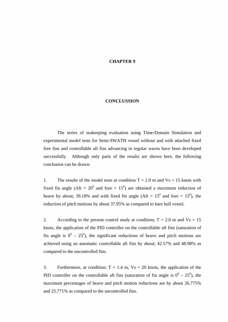
CHAPTER 9
CONCLUSSION
The series of seakeeping evaluation using Time-Domain Simulation and
experimental model tests for Semi-SWATH vessel without and with attached fixed
fore fins and controllable aft fins advancing in regular waves have been developed
successfully. Although only parts of the results are shown here, the following
conclusion can be drawn:
1. The results of the model tests at condition T = 2.0 m and Vs = 15 knots with
fixed fin angle (Aft = 200 and fore = 150) are obtained a maximum reduction of
heave by about; 39.18% and with fixed fin angle (Aft = 150 and fore = 150), the
reduction of pitch motions by about 37.95% as compared to bare hull vessel.
2. According to the present control study at condition; T = 2.0 m and Vs = 15
knots, the application of the PID controller on the controllable aft fins (saturation of
fin angle is 00 – 250), the significant reductions of heave and pitch motions are
achieved using an automatic controllable aft fins by about; 42.57% and 48.98% as
compared to the uncontrolled fins.
3. Furthermore, at condition; T = 1.4 m, Vs = 20 knots, the application of the
PID controller on the controllable aft fins (saturation of fin angle is 00 – 250), the
maximum percentages of heave and pitch motion reductions are by about 26.775%
and 25.771% as compared to the uncontrolled fins.
189
CHAPTER 10
FUTURE RESEARCH
1. It will good basis for naval architects to design a suitable controllable fin
for a Semi-SWATH vessel in irregular seas.
2. Although the present control technique here is conventional PID
controller theory shows a good results regarded as useful for basic
controller reference results. In fact, the present control theory can be
incorporated with a modern control theories, e.g. fuzzy control, ANN
control, LQG control or adaptive control, etc., to make the fin control
even more effective and robust. In other words, the analytical tool
developed here may offer very useful information to the Semi-SWATH
vessel designers in case automatic controllable fins.
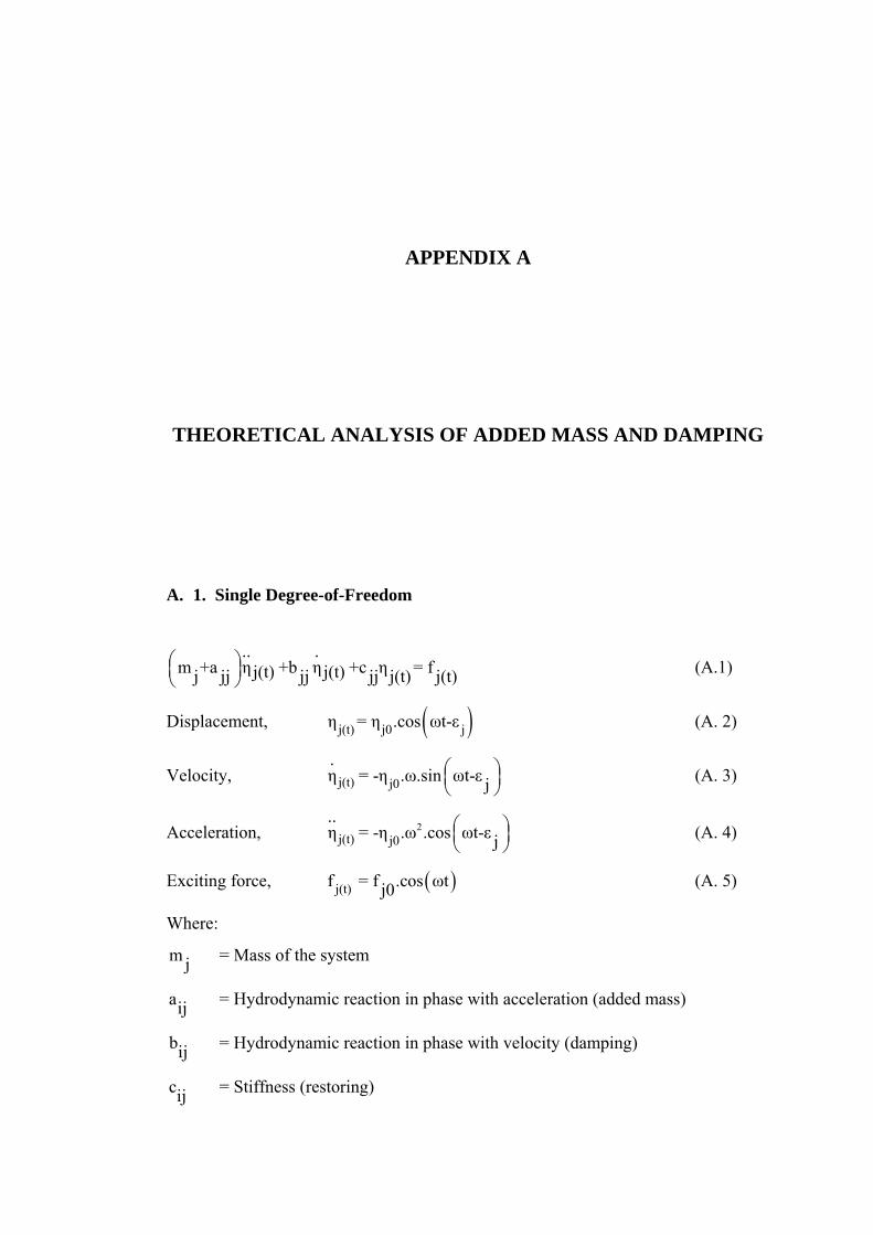
APPENDIX A
THEORETICAL ANALYSIS OF ADDED MASS AND DAMPING
A. 1. Single Degree-of-Freedom
.. .
m +a η +b η +c η = fj(t) j(t)j jj jj jj j(t) j(t)⎛ ⎞⎜ ⎟⎝ ⎠
(A.1)
Displacement, ( )j(t) j0 jη = η .cos ωt-ε (A. 2)
Velocity, j(t) j0
.η = -η .ω.sin ωt-ε j
⎛ ⎞⎜ ⎟⎝ ⎠
(A. 3)
Acceleration, 2j(t) j0
..η = -η .ω .cos ωt-ε j
⎛ ⎞⎜ ⎟⎝ ⎠
(A. 4)
Exciting force, ( )j(t)f = f .cos ωtj0 (A. 5)
Where:
m j = Mass of the system
aij = Hydrodynamic reaction in phase with acceleration (added mass)
bij = Hydrodynamic reaction in phase with velocity (damping)
cij = Stiffness (restoring)
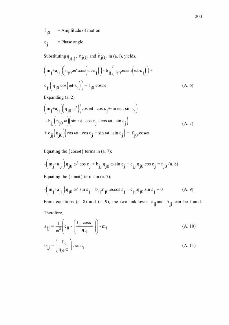
200
f j0 = Amplitude of motion
ε j = Phase angle
Substitutingη j(t) , .η j(t) and
..η j(t) in (a.1), yields,
( ) ( )2m +a η .ω .cos ωt-ε - b η .ω.sin ωt-ε +j ij j0 j jj j0 j⎛ ⎞ ⎛ ⎞⎛ ⎞⎜ ⎟⎜ ⎟ ⎜ ⎟⎝ ⎠⎝ ⎠ ⎝ ⎠
( )c η .cos ωt-ε = f .cosωtjj j0 j j0⎛ ⎞⎜ ⎟⎝ ⎠
(A. 6)
Expanding (a. 2)
( )( )( )( )( )( )
2m +a η .ω cos ωt . cos ε +sin ωt . sin ε j ij j0 j j
- b η .ω sin ωt . cos ε - cos ωt . sin εjj j0 j j
+ c η cos ωt . cos ε + sin ωt . sin ε = f .cosωtjj j0 j j j0
⎛ ⎞⎜ ⎟⎝ ⎠
(A. 7)
Equating the ( )cosωt terms in (a. 7);
2- m +a .η .ω .cos ε + b .η .ω.sin ε + c .η .cos ε = fj ij j0 j jj j0 j jj j0 j j0⎛ ⎞⎜ ⎟⎝ ⎠
(a. 8)
Equating the ( )sinωt terms in (a. 7);
2- m +a .η .ω .sin ε + b .η .ω.cos ε + c .η .sin ε = 0j ij j0 j jj j0 j jj j0 j⎛ ⎞⎜ ⎟⎝ ⎠
(A. 9)
From equations (a. 8) and (a. 9), the two unknowns aij and b jj can be found.
Therefore,
j0 jjj j2
j0
f .cosε1a = c - - mjj ηω
⎛ ⎞⎛ ⎞⎜ ⎟⎜ ⎟⎜ ⎟⎜ ⎟⎝ ⎠⎝ ⎠
(A. 10)
j0j
j0
fb = . sinεjj η .ω
⎛ ⎞⎜ ⎟⎜ ⎟⎝ ⎠
(A. 11)
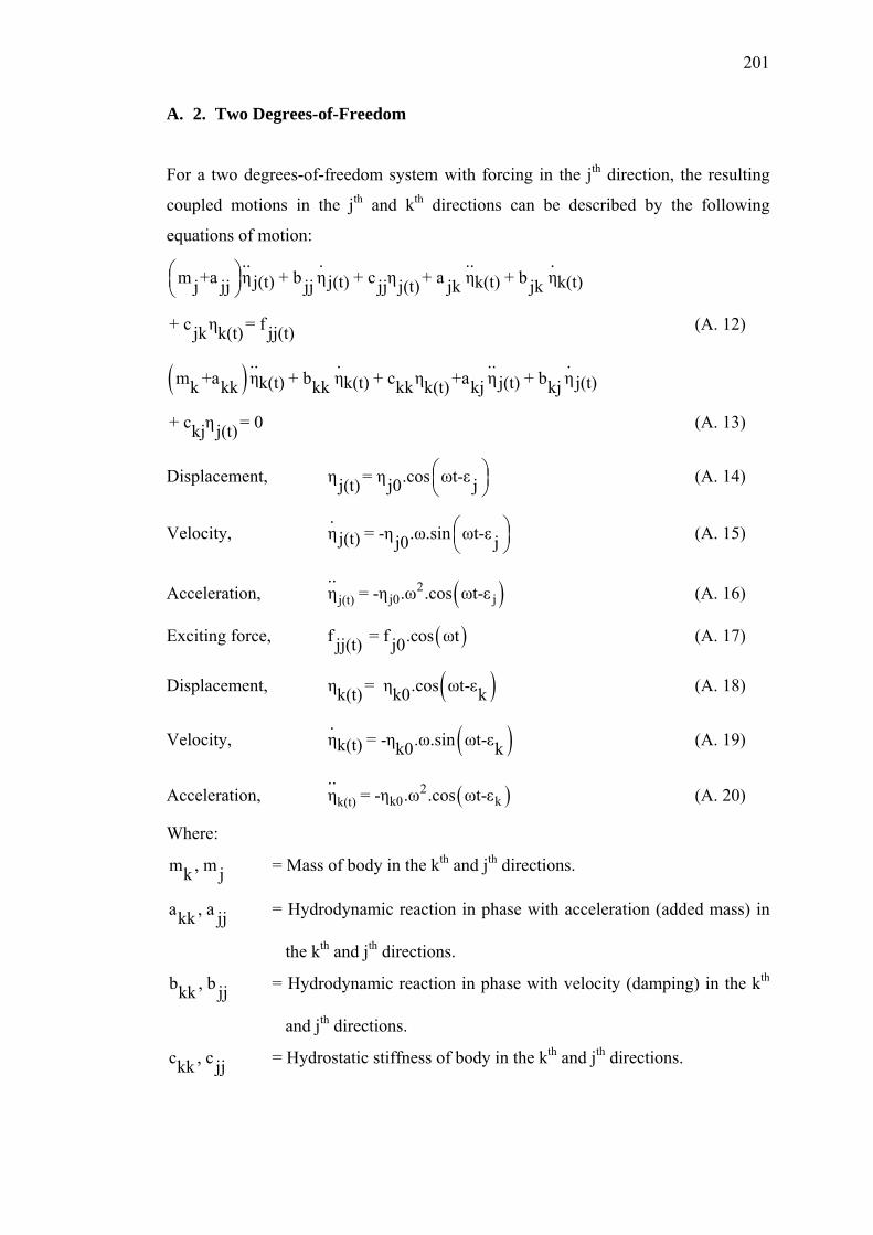
201
A. 2. Two Degrees-of-Freedom
For a two degrees-of-freedom system with forcing in the jth direction, the resulting
coupled motions in the jth and kth directions can be described by the following
equations of motion: .. . .. .
m +a η + b η + c η + a η + b ηj(t) j(t) k(t) k(t)j jj jj jj j(t) jk jk⎛ ⎞⎜ ⎟⎝ ⎠
+ c η = fjk k(t) jj(t) (A. 12)
( ) .. . .. .m +a η + b η + c η +a η + b ηk(t) k(t) j(t) j(t)k kk kk kk k(t) kj kj
+ c η = 0kj j(t) (A. 13)
Displacement, η = η .cos ωt-εj(t) j0 j⎛ ⎞⎜ ⎟⎝ ⎠
(A. 14)
Velocity, .η = -η .ω.sin ωt-εj(t) j0 j
⎛ ⎞⎜ ⎟⎝ ⎠
(A. 15)
Acceleration, ( )2j0 jj(t)
..η = -η .ω .cos ωt-ε (A. 16)
Exciting force, ( )f = f .cos ωtjj(t) j0 (A. 17)
Displacement, ( )η = η .cos ωt-εk(t) k0 k (A. 18)
Velocity, ( ).η = -η .ω.sin ωt-εk(t) k0 k (A. 19)
Acceleration, ( )2k0 kk(t)
..η = -η .ω .cos ωt-ε (A. 20)
Where:
m , mk j = Mass of body in the kth and jth directions.
a , akk jj = Hydrodynamic reaction in phase with acceleration (added mass) in
the kth and jth directions.
b , bkk jj = Hydrodynamic reaction in phase with velocity (damping) in the kth
and jth directions.
c , ckk jj = Hydrostatic stiffness of body in the kth and jth directions.
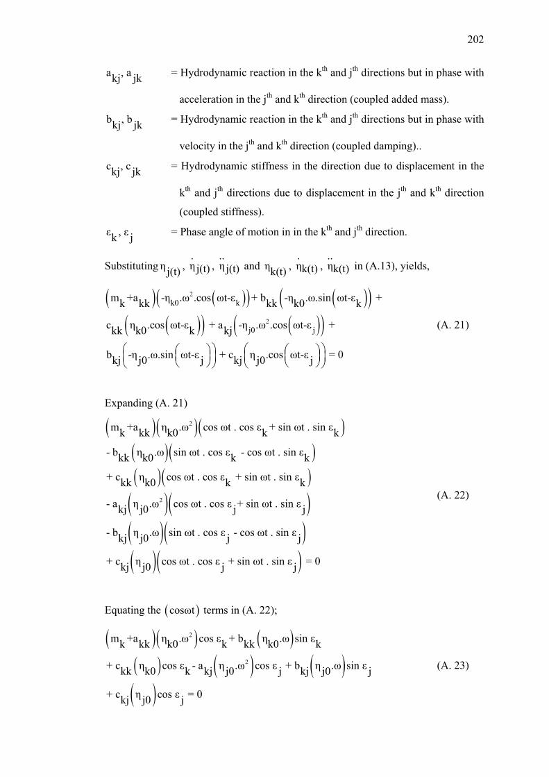
202
a , akj jk = Hydrodynamic reaction in the kth and jth directions but in phase with
acceleration in the jth and kth direction (coupled added mass).
b , bkj jk = Hydrodynamic reaction in the kth and jth directions but in phase with
velocity in the jth and kth direction (coupled damping)..
c , ckj jk = Hydrodynamic stiffness in the direction due to displacement in the
kth and jth directions due to displacement in the jth and kth direction
(coupled stiffness).
ε , εk j = Phase angle of motion in in the kth and jth direction.
Substitutingη j(t) , .η j(t) ,
..η j(t) and ηk(t) ,
.ηk(t) ,
..ηk(t) in (A.13), yields,
( ) ( )( ) ( )( )( )( ) ( )( )
2
2
k0 k
j0 j
m +a -η .ω .cos ωt-ε + b -η .ω.sin ωt-ε + k kk kk k0 k
c η .cos ωt-ε + a -η .ω .cos ωt-ε + kk k0 k kj
b -η .ω.sin ωt-ε + c η .cos ωt-ε = 0kj j0 j kj j0 j⎛ ⎞ ⎛ ⎞⎛ ⎞ ⎛ ⎞⎜ ⎟ ⎜ ⎟⎜ ⎟ ⎜ ⎟⎝ ⎠ ⎝ ⎠⎝ ⎠ ⎝ ⎠
(A. 21)
Expanding (A. 21)
( )( )( )( )( )( )( )( )( )( )
2
2
m +a η .ω cos ωt . cos ε + sin ωt . sin ε k kk k0 k k
- b η .ω sin ωt . cos ε - cos ωt . sin εkk k0 k k
+ c η cos ωt . cos ε + sin ωt . sin ε kk k0 k k
- a η .ω cos ωt . cos ε + sin ωt . sin ε kj j0 j j
- b η .ω sin ωt . cos ε kj j0 j( )( )( )
- cos ωt . sin ε j
+ c η cos ωt . cos ε + sin ωt . sin ε = 0kj j0 j j
(A. 22)
Equating the ( )cosωt terms in (A. 22);
( )( ) ( )( ) ( ) ( )( )
2
2
m +a η .ω cos ε + b η .ω sin εk kk k0 k kk k0 k
+ c η cos ε - a η .ω cos ε + b η .ω sin ε kk k0 k kj j0 j kj j0 j
+ c η cos ε = 0kj j0 j
(A. 23)
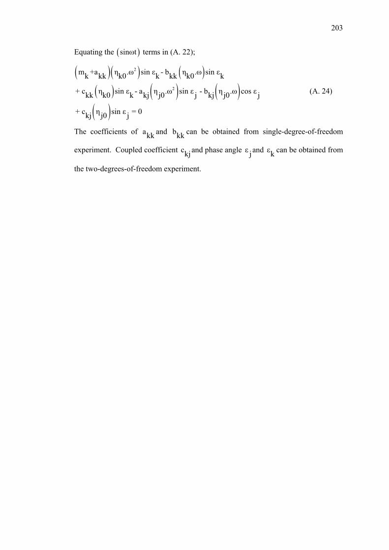
203
Equating the ( )sinωt terms in (A. 22);
( )( ) ( )( ) ( ) ( )( )
2
2
m +a η .ω sin ε - b η .ω sin εk kk k0 k kk k0 k
+ c η sin ε - a η .ω sin ε - b η .ω cos ε kk k0 k kj j0 j kj j0 j
+ c η sin ε = 0kj j0 j
(A. 24)
The coefficients of akk and bkk can be obtained from single-degree-of-freedom
experiment. Coupled coefficient ckjand phase angle ε jand εk can be obtained from
the two-degrees-of-freedom experiment.
APPENDIX B
MATLAB ODE
1. ode45
Ode45 is based on an explicit Runge-Kutta (4,5) formula, the Dormand-
prince pair. It is, a one-step solver; that is, in computing y(tn), it needs only the
solution at the immediately preceding time point, y(tn-1). In general, ode45 is the
best solver to apply as a first try for most problems. For this reason, ode45 is the
default solver used by Simulink for models with continuous states.
2. ode23
ode23 is also based on an explicit Runge-Kutta (2,3) pair of Bogacki and
Shampine. It can be more efficient than ode45 at crude tolerances and in the presence
of mild stiffness. Ode23 is a one-step solver.
3. ode113
ode113 is a variable order Adams-Bashforth-Moulton PECE solver. It may be
more efficient than ode45 at stringent tolerances and when the ODE file function is
particularly expensive to evaluated, ode113 is a multistep solver – it normally needs
the solutions at several preceding time points to compute the current solution.
205
4. ode15s
ode15s is a variable order solver based on the numerical differentiation
formulas (NDFs). These are related to but are more efficient than the backward,
BDFs (also known as a Gear’s method). Like ode113, ode15s is a multistep method
solver. If you suspect that the problem is stiff, or if ode45 failed or was very
inefficient, try ode15s.
5. ode23s
ode23s is based on modified Rosenbrock formula of order 2. Because it is
one-step solver, it can be more efficient than ode15s at crude tolerances. It can solve
some kinds of stiff problems for which ode 15s are not effective.
6. ode23t
ode23t is an implementation of the trapezoidal rule using a”free” interpolant.
Use this solver if the problem is only moderately stiff and you need a solution
without numerical damping.
7. ode23tb
ode23tb is an implementation of the TR-BDF2, an implicit Runge-Kutta
Merson formula with a first stage that is trapezoidal rule step and a second stage that
is a backward differentiation formula of order two. By construction, the same
iteration matrix is used in evaluating both stages. Like ode23s, this solver can be
more efficient than ode15s at crude tolerances.
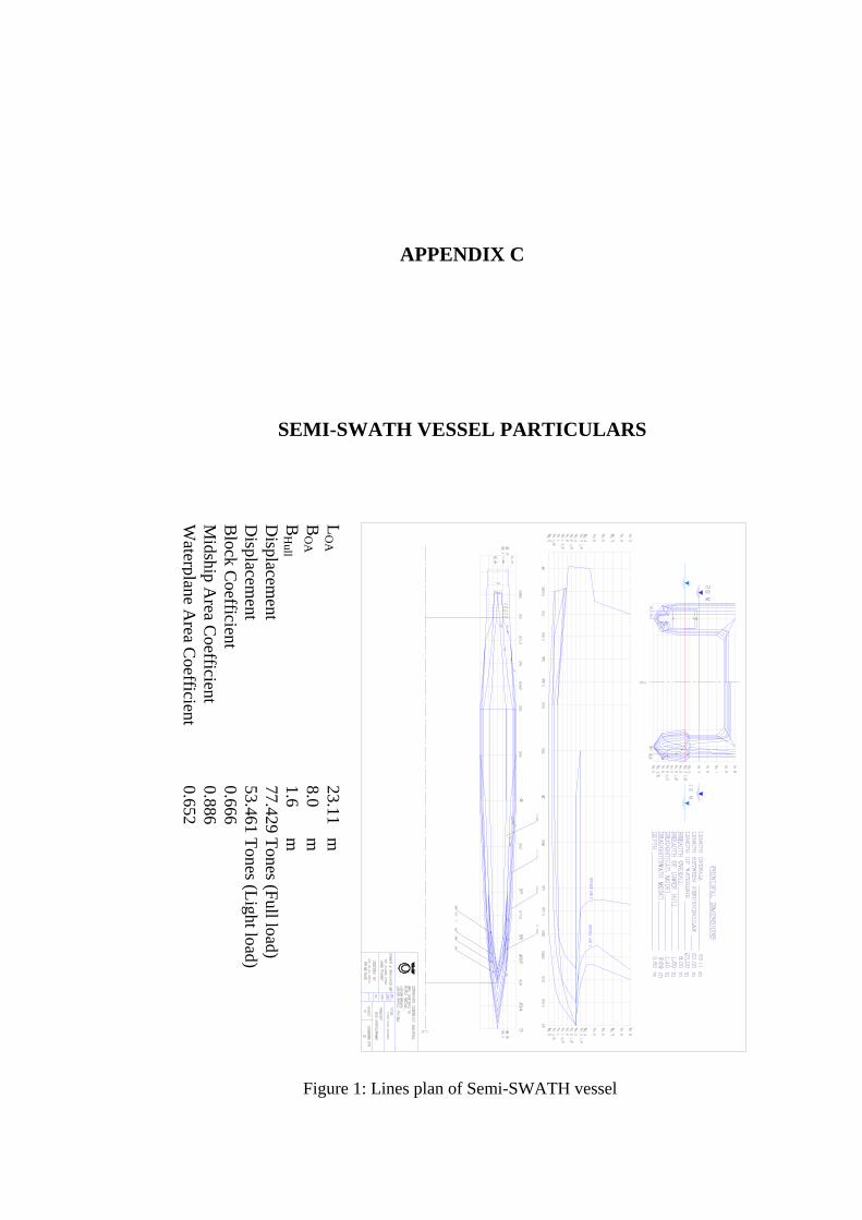
APPENDIX C
SEMI-SWATH VESSEL PARTICULARS
LO
A
23.11
m
BO
A
8.0
m
BH
ull
1.6
m
Displacem
ent
77.429 Tones (Full load)
Displacem
ent
53.461 Tones (Light load)
Block C
oefficient
0.666
Midship A
rea Coefficient
0.886
Water plane A
rea Coefficient
0.652
Figure 1: Lines plan of Semi-SWATH vessel
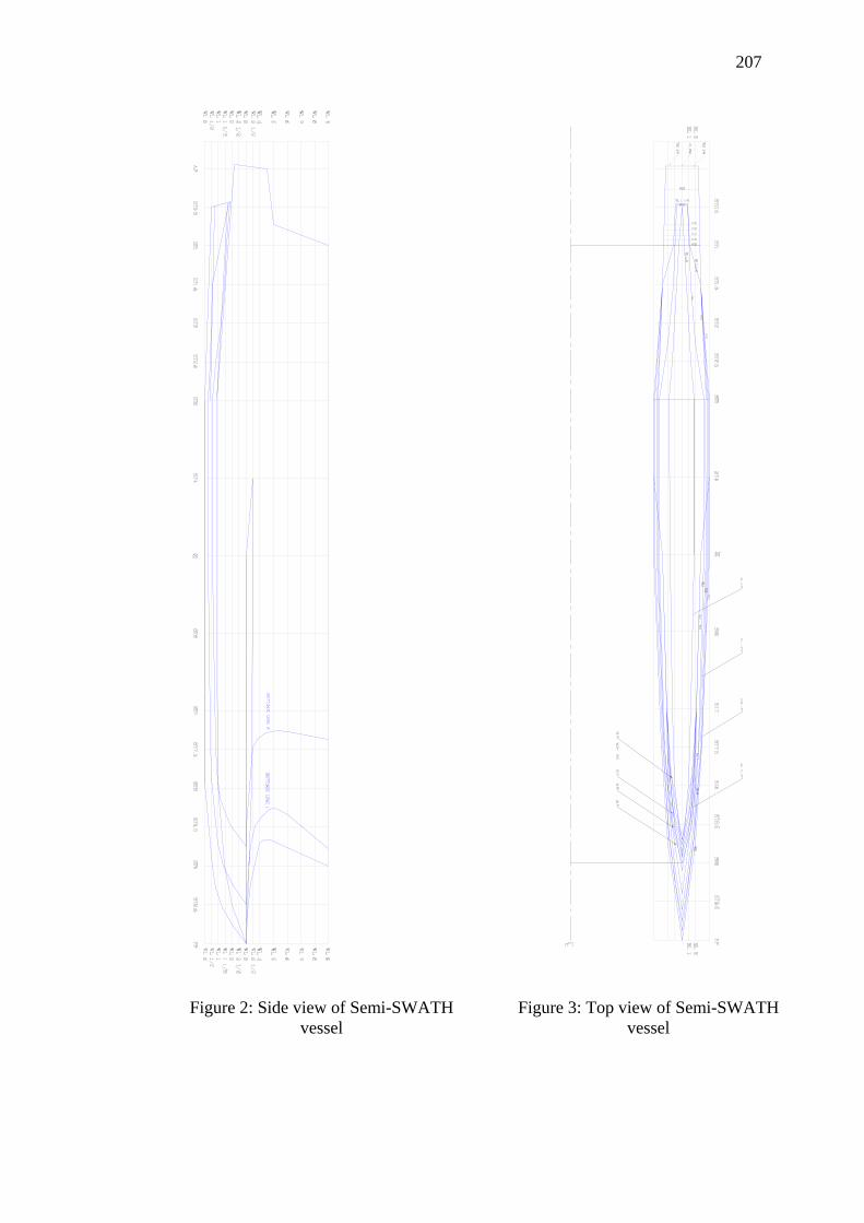
207
Figure 2: Side view of Semi-SWATH vessel
Figure 3: Top view of Semi-SWATH vessel
Figure 2: Side view of Semi-SWATH vessel
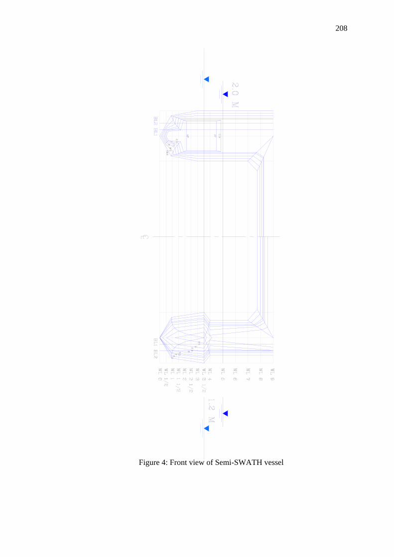
208
Figure 4: Front view of Semi-SWATH vessel
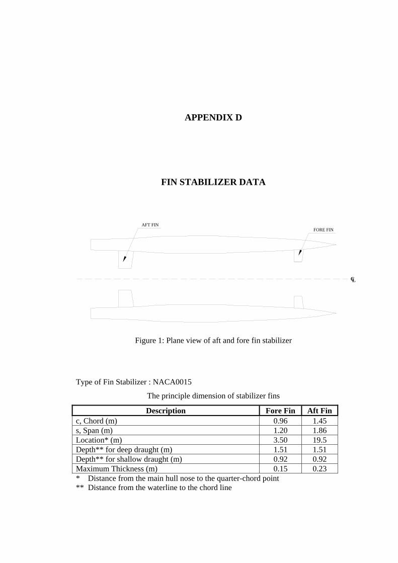
APPENDIX D
FIN STABILIZER DATA
Figure 1: Plane view of aft and fore fin stabilizer
Type of Fin Stabilizer : NACA0015
The principle dimension of stabilizer fins
Description Fore Fin Aft Fin c, Chord (m) 0.96 1.45 s, Span (m) 1.20 1.86 Location* (m) 3.50 19.5 Depth** for deep draught (m) 1.51 1.51 Depth** for shallow draught (m) 0.92 0.92 Maximum Thickness (m) 0.15 0.23 * Distance from the main hull nose to the quarter-chord point ** Distance from the waterline to the chord line
AFT FIN
LC
FORE FIN
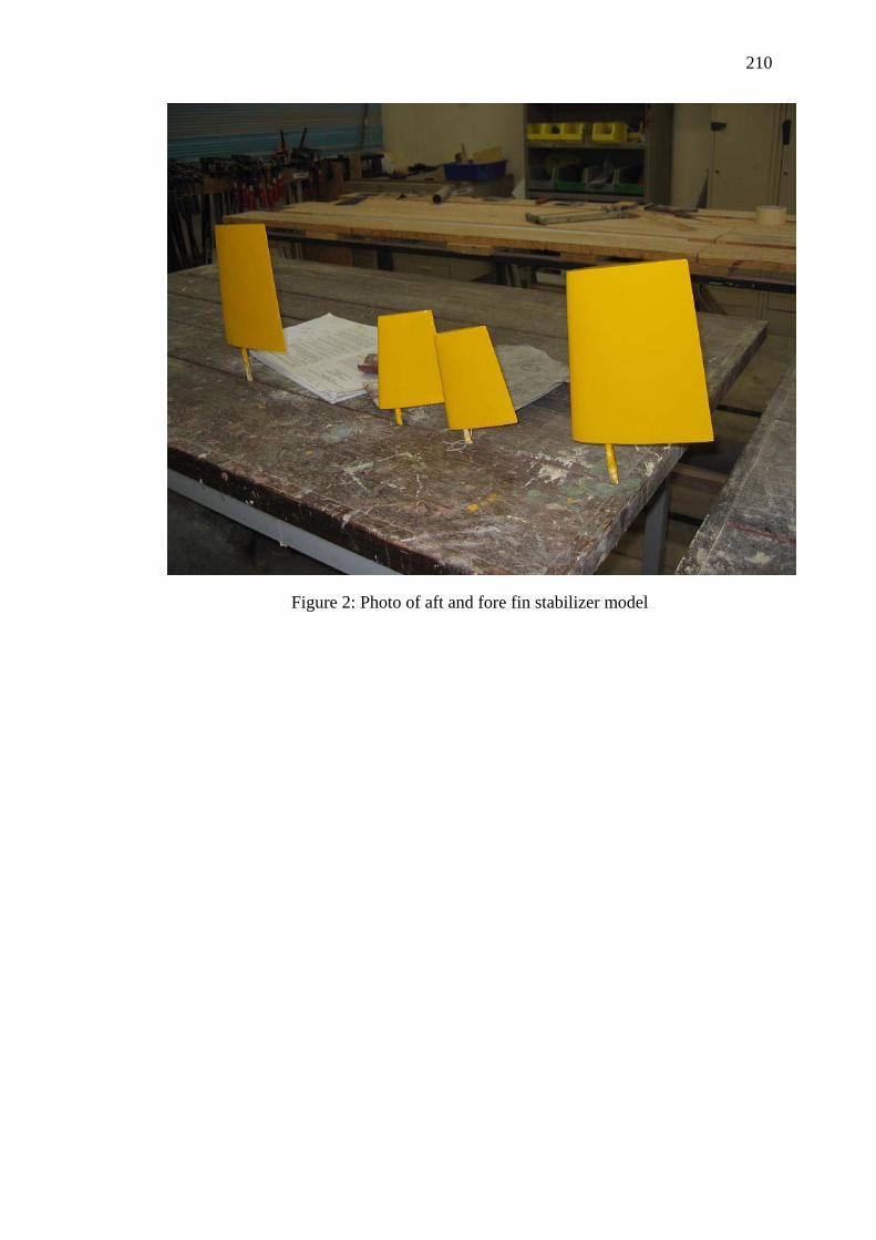
210
Figure 2: Photo of aft and fore fin stabilizer model
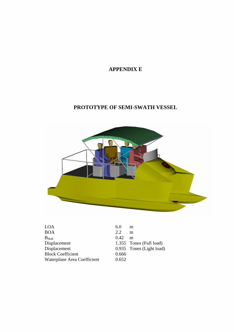
APPENDIX E
PROTOTYPE OF SEMI-SWATH VESSEL
LOA 6.0 m BOA 2.2 m BHull 0.42 m Displacement 1.355 Tones (Full load) Displacement 0.935 Tones (Light load) Block Coefficient 0.666 Waterplane Area Coefficient 0.652
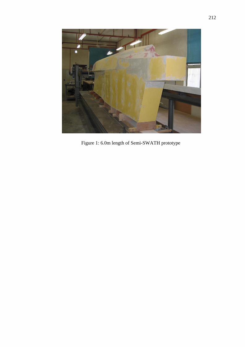
212
Figure 1: 6.0m length of Semi-SWATH prototype
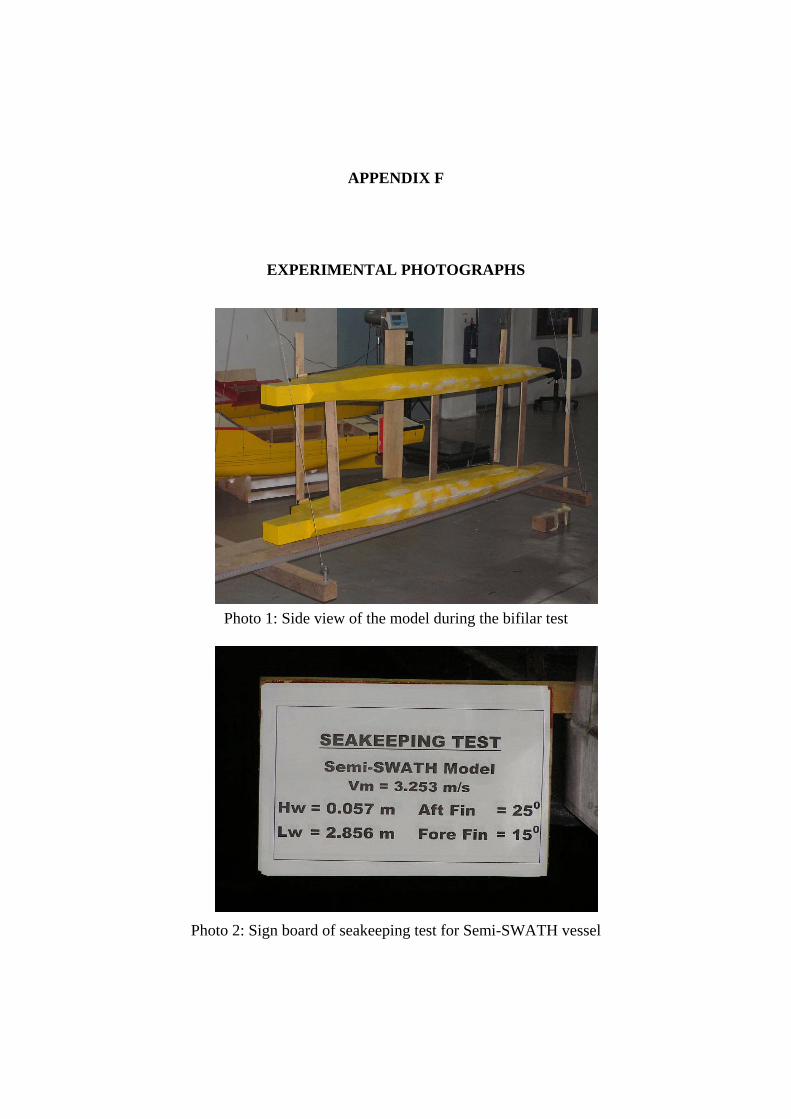
APPENDIX F
EXPERIMENTAL PHOTOGRAPHS
Photo 1: Side view of the model during the bifilar test
Photo 2: Sign board of seakeeping test for Semi-SWATH vessel
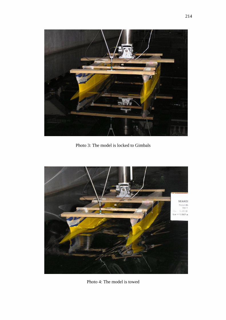
214
Photo 3: The model is locked to Gimbals
Photo 4: The model is towed
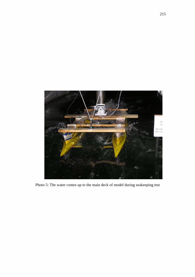
215
Photo 5: The water comes up to the main deck of model during seakeeping test
REFERENCES
A. Lloyd (1989). “Seakeeping Behavior in Rough Weather”, Ellis Horwood Ltd.
Abkowitz, M. A., (1959). “The Effect of Anti-Pitching Fins on Ship Motions”, Trans
SNAME, Vol. 67, pp. 210-252.
Aström, K. J., and Hagglund, T (1984). ”Automatic Tuning of Simple regulators
with Specifications on phase and amplitude margins,” Automatica, 20, pp.
645-651.
Atlar, M. (1982). “A Study of Frank Close Fit Method, Theory, Application and
Comparison with Other Methods”. Report No: NAOE-HL-81-08, University
of Glasgow.
Beena, V.I. and Subramanian, V.A. (2003). “Parametric studies on seaworthiness of
SWATH Ships”. London: Elsevier. Vol. 30, pp. 1077-1106.
Bhattacarya, R. (1978). “Dynamic of Marine vehicles”. John Wiley and Sons.
Buang Ain, V., (2001). “Computer Aided Calculation of Hydrodynamic Coefficients
of Simple Hull Section”, Universiti Teknologi Malaysia. Bachelor
Research.
Caldeira, S. F., and Clarke, D., (1988). “The Active Control of SWATH Motions”,
Proceeding, International Conference of SWATH Ships and Advanced Multi-
Hull Vessels II, RINA, May, Southampton, UK.
191
Chen, W. C., et. al, (1995). “Study on the Pitching Motion Reduction for a Fast Ship
in Waves ”, Trans SNAME, 8th Symposium of SNAME, pp. 80-85.
Chinn, N. L., et. al, (1994) “Mathematical Modelling of a Small Waterplane Area
Twin Hulled (SWATH) Vessel”, pp. 1560-1565.
Chun, H. H., and McGregor, R. C (1995). “Development of a Practical SWATH ship
with High Performance”, PRADS ‘95, Hyundai Maritime Research Institute
(Korea) and Dept. of Mechanical Engineering, Glasgow University (U.K), pp
1313-1321.
Coburn, J. L., et al., (1999). “Design of SWATH Coastal Research Vessel”, Institute
of Electrical & Electronics Engineers, Vol. 1, pages 526-542.
Conolly, J. E., and Goodrich, G. L., (1968). “Sea Trial of Anti-Pitching Fin”, pp. 87-
100.
Davis, M. R., and Holloway, D. S., (2003). “The Influence of Hull Form on The
Motions of High-Speed Vessels in Head Seas”, Elsevier Science Publisher,
Ocean Engineering Vol. 30, pp. 2091-2115.
Djatmiko, E. B., (2004). “Effect of Stabilizing Fins On The SWATH Ship Heave
And Pitch Motion Characteristics”, Malaysia, Martech 4th Regional
Conference. Vol. 4, pp. 14-40.
Dubrovskiy, V. A., (2000). “Complex Comparison of Seakeeping: Method and
Example”, Marine Technology and SNAME News, October 2000, Vol. 37,
No. 4, pp. 223-229.
Dubrovskiy, V. A., and Lyakhoviyskiy, A., (2001). “Multi-Hull Ships”, Backbone
Publishing Company, United States of America, USA, pp. 225.
Esteban, S., et al, (1999). “Predictive Perturbation Cancelling For Seakeeping
Improvement Of A Fast Ferry”, Departamento de Arquitectura de
192
Computadores y Automatica, Facultad de Fisicas, Universidad Complutense
de Madrid, Ciudad Universitaria. 28040 Madrid, Spain.
Esteban, S., et. al, (2000). “A Computer-Based Tesbed For Designing The Control of
Vertical Motions of a Fast Ferry”, Departamento de Arquitectura de
Computadores y Automatica, Facultad de Fisicas, Universidad Complutense
de Madrid, Ciudad Universitaria. 28040 Madrid, Spain.
Fairlie-Clark, A.C., et al (1990). “On the Design and Evaluation of Control System
for SWATH ship”, Exeter, UK: Proceeding, International Conference on
Modeling and Control Marine Craft, pp. 53-74.
Fang, M. C, and Kim, C. H, (1986). “Hydrodynamically Coupled Motion Two Ships
Advancing in Oblique Seas”, Journal of Ship Research, Vol. 30, pp. 159-171.
Fang, M. C., (1988) “The Motions of SWATH ships in Waves”, Journal of Ship
Research, Vol. 32, pp. 238-245.
Fang, M. C., and Lin, B, L., (1995). “The Simulation of The SWATH Ship Motion
With Fixed Fin In Longitudinal Waves”, 5th Proceeding International
Offshore and Polar Engineering Conference, June, The Hague, Netherlands,
Vol. III, pp. 484-491.
Fang, M. C., and Lin, B. N., (1998). “The Simulation of The SWATH Ship Motion
With Controllable Fin In Longitudinal Waves”, International Shipbuilding
Progress, Vol. 45, pp. 283-307.
Fossen, T. J., (1994). “Guidance and Control of Ocean Vehicles”, New York, Willey.
G. Khristoffer., (2002). “Prediction of Slamming Occurrence of Catamarans”, Master
Thesis, Curtin University of Technology.
Gaul, D. R., et al. (1988). “Design of a Semi-Submerged SWATH Research and
Survey Ship”, Proceedings of OCEANS ’88, Conference in Baltimore,
Maryland, pp. 1149-1156.
193
Gaul, D. R., et al., (1979). “The Use of Semi-Submerged to Support New
Technology at Sea”, IEEE, CH1478-7, pp. 159-166.
Gaul, R. D., and McClure, A. C., (1984). “Development of the SWATH Ship
Concept for Research Ship Design”, Proceedings of OCEANS ‘84,
Conference in Washington, D.C., September, pp. 10-12.
Giron-Sierra, J. M., et. al., (2002). “The Control of Specific Actuators For Fast Ferry
Vertical Motion Damping”, IEEE International Symposium on Computer
Aided Control System Design Proceedings, Glasgow, Scotland, U. K., pp. 1-
63.
Goodyear, J. E., et al., (1989). “An Evaluation of The SWATH Vessel Frederrick G.
Creed in The Canadian North Atlantic”, Supplied by British Library, pp 109-
112.
Grande, G., (2002). “Prediction of Slamming Occurrence of Catamarans”, Master
Thesis, Curtin University of Technology.
GrØnnslett, K. A., et al., (1987). “Design Charts For High-Speed Catamaran”, pp.
91-96.
Hadler, J. B., et al., (1974). “Ocean Catamaran Seakeeping Design Based On the
Experiences of USNS Hayes”, Transaction of SNAME. Vol. 82, pp 127-161.
Hannon, M., and Andrenilson, M. R., (2000). “Behaviour of a High Speed
Catamaran in Following Seas”, International Conference on Ships and
Shipping Research, Venice (ITALIA).
Haywood, A. J., et al (1995) .“The Development of a Ride Control System for Fast
Ferries” IFAC Control Engineering Practice, pp. 695-703.
194
Holloway, D. S., and Davis, M. R., (2003). “Seakeeping Computations of Semi-
SWATHs at High Froude Number”, The University of Tasmania GPO Box
252-65 HOBART, TAS 7001 AUSTRALIA, pp. 1-21.
Holloway, D. S., and Davis, M. R., (2003). “Experimental Seakeeping of Semi-
SWATHs at Intermediate to High Froude Numbers”, The University of
Tasmania, pp. 1-18.
Holloway, D. S., (2003). “Experimental Seakeeping of Semi-SWATH ship at High
Froude Number”, University of Tasmania, Australia, Trans RINA, pp. 15-30.
Holloway, D. S., (1998). “A High Froude Number Time Domain Strip Theory
Applied to the Seakeeping of Semi-SWATHs”, PhD Thesis, University of
Tasmania.
Hong, Y. S., (1980). “Improvements in The Prediction of Heave and Pitch Motion
for SWATH Ships”, DTNSRDC Departmental report SDR0928-02,
Bethesda.
Jingyi, W., and Yinhai, F., (2001). “A Fuzzy PID controller for ship course based
on engineering tuning methods” IEEE,0-7803-7010-4, pp. 376-381.
Kallio, J. A., and Ricci, J. J., (1976). “Seaworthiness Characteristics of A Small
Waterplane Area of Twin-Hull”, (SWATH IV) Part II, DTNRSDC Report
SPD 620-02.
Kamlesh S. et al., (2000). “Motions and Slamming Impact on Catamaran”
Department of Naval Architecture and Ocean Engineering, University of
Glasgow, Acre Road Glasgow G12 8QQ, UK. Ocean Engineering Vol.27, pp.
729–747.
Kang, C., and Gong, I., (1995). “Time-Domain Simulation of The Motion of a High-
Speed Twin-Hull With Control Planes in Waves”, 3rd Proceeding, Fast95,
International Conference on Fast Transportation, October, Germany, pp.
1031-1041.
195
Kenevissi, F., et al., (2003). “A New- Generation Motion-Control System for Twin-
Hull Vessels Using a Neural Optimal Controller”, Journal of Marine
Technology, Vol. 40, pp. 168-180.
Kennell, C., (1992). “SWATH Ships”, USA: The Society Of Naval Architects And
Marine Engineers. Technical and Research Bulletin. No. 7-5.
Kim, S. H., and Yamato, H., (2004). “On The Design of a Longitudinal Motion
Control System of a Fully-Submerged Hydrofoil Craft Based on Optimal
Preview Servo System”, Elsevier Science Publisher, Ocean Engineering, Vol
31, pp. 1637-1653.
Korvin-Kroukovski, B. V., and Jacobs, W. R., (1957). “Pitching and Heaving
Motions of a Ship in Reguler Waves”, SNAME Trans., 65, pp. 590-632.
Lang, T., G. et al (1988). “A Transport and System Deployment Concept for Near
Shore Mine Warfare”, Blue Sea Corporation, Houston, Texas, pp. 1-10.
Lee, C. M., (1976) .“Theoretical Prediction of Motion of Small Waterplane Area,
Twin-Hull (SWATH) in Waves”, DTNSRDC report 76-004, Bethesda.
Lewis, C. H., and Griffin, M. J., (1997). “Evaluating The Motions of Semi-
Submersible With Respect to Human Response”, Elsevier Science Ltd,
Applied Ergonomics Vol28, No. 3, pp 193-201.
Liu, D., and Wong, K. M., (1986). “Development and Analysis of SWATH Ships”,
pp II. b-1.
Maimun, A., (1993). “Stability of Fishing Vessels in Astern Sea-Shallow Water
Environment”, Ph. D. Thesis. Dept. Of Ship and Marine Technology,
University of Strathclyde.
196
McCreight, K. K., (1987). “Assessing the Seaworthiness of SWATH ships”.
Transaction of SNAME, Vol. 95, pp 189-214.
McGregor, R. C., (1992). “At The Potential of SWATH Ships”, Department of
Mechanical Engineering, University of Glasgow, Glasgow, G128QQ,
Scotland, UK, pp. 197.
Min, K. S., et al., (1987). “Conceptual Design of Very Large-Size Super-High-Speed
Foil Catamaran Containership”, Heavy Industries Co., Ltd., 1, Cheon-Ha
Dong, Dong-Ku, Ulsan, KOREA, pp. 1-8.
Murthy, T. K. S,. “Extended Performance of SWATH ship”, Naval Architect and
SSACV Development Consultant, pp. 32-38.
Neng, T., et. al., (1999). “Control System Design and Performance Evaluation Anti-
pitching Fins”, SNAJ Publisher, Journal Marine Science and Technology,
Vol. 4, pp. 117-122.
O’Hanlon, J. F., and McCauley, M. E., (1974). “Motion sickness incidence as a
function of acceleration of vertical sinusoidal motion”, Aerospace Medicine
45 (4), 366–369.
Ohmatsu, S., Yoshino, T., Yamamoto, T., Ishida, S., Nimura, T., Sugai, K., (1983).
“An experimental study on the motion control of semi-submerged ships”,
Journal of the Society of Naval Architects of Japan 152, 229–238.
Ozawa, H., (1987). “The Design and Operation of Catamaran Vessels”, Mitsui
Engineering and Shipbuilding Coefficient. Ltd, pp. 139-155.
Papanikolaou, A, et al., (1997). “Hydrodynamic Optimization of Fast-Displacement
Catamarans”, National Technical University of Athens, Greece, pp. 697-714.
197
Papanikolaou, D. A., (1991). “Computer-Aided Preliminary Design of a High Speed
SWATH Passanger Ferry”, 4th International Marine Systems Design
Conference, pp. 75-89.
Pinto, S. G. et al., (2001). “Implementation of High-Order Implicit Runge-Kutta
Methods”, Journal of Computers and Mathematics for Applications.
Pergamon, Vol. 41, pp. 1009-1024.
Renilson, M. R. and Anderson. V., (2002). “Deck Diving of Catamarans in
Following Seas”, Fast 97 International Conference on Fast Sea
Transportation, Australia.
Salvesen, N., Tuck, E. O. and Jacobs, W. R. (1970). “Ship Motions and Sea Loads”,
SNAME Trans., 78, pp. 250-285.
Sariöz, K., and Narli, E., (2005). “Effect of Criteria on Seakeeping Performance
Assessment”, Ocean Engineering, Vol. 27, pp. 1161-1173.
Segundo, E., et al., (2000). “Smoothing Fast Ferry Vertical Motions: A
Simulationenvironment For The Control Analysis”, Dept. Arquitectura de
Computadores y Automatica, Facultad de Ciencias Físicas Universidad
Complutense de Madrid, 28040 Madrid, Spain.
Shack, C., (1995). “Research on Semi-SWATH Hull Forms”, 3rd Proceeding, Fast95,
3rd International Conference on Fast Transportation, October, Germany, pp.
527-538.
Shigehiro, R., and Kuroda, T., (2000). “Effect of Anti-Pitching Fins on Ship’s
Motions by the Methods of Evaluation Passengers Comfort”, ISOPE’2000,
Seattle, WA, USA.
Surendrana, S., et al., (2006). “Studies On An Algorithm To Control The Roll
Motion Using Active Fins” Journal of Ocean Engineering, pp. 1-10.
198
Vugts, J. H., (1967). “Pitch and Heave with Fixed and Controlled Bow Fins”,
International Shipbuilding Progress, Vol. 14, pp. 191-215.
Ware, J. R., Best, J. F., and Scott, V. A., (1980b). “Application of Optimal Control
Techniques to SWATH vertical Plane Control”, DTNSRDC, Bethesda,
March, ORI TR No. 1682.
Ware, J. R., Best, J. F., and Scott, V. A., (1981). “SWATH Optimal Control Design
Using Optimal Techniques”, Proceeding, 6th Ship Control System
Symposium, DTNSRDC, October, Ottawa, Canada.
Warlee, F. V., and Luth, H. R., (2000). “Scale Effect on Foils and Fins in Steady and
Unsteady Flow”, Hydrodynamic of High Speed Craft 2000, Trans RINA, pp.
1-8.
Wu, J. Y., (1984). “A Study of The Effect of Fin Size on The Pitch And Heave
Motion of A SWATH Ship”, NAOE-84-55 Report, Department Of Naval
Architecture And Ocean Engineering, University of Glasgow.
Wu, J. Y., and McGregor, R. C., (1985). “ SWATH Seakeeping in The Presence of
Control Fins”, Proceeding, 5th High-Speed Surface Craft Conference, May,
Southampton, UK, pp. 97-112.
Zarnick, E. E., (1998). “SWATH Ship Motion Control With Active Fins”, RINA
International Conference on SWATH Ships and Advanced multi-hulled
vessels, London, U.K.
Ziegler, J, G and Nichols, N, B., (1942). “Optimum Settings For Automatic
Controllers”, Trans. ASME, pp. 759–768.
UNIVERSITI TEKNOLOGI MALAYSIA
UTM/RMC/F/0024 (1998)
BORANG PENGESAHAN
LAPORAN AKHIR PENYELIDIKAN
TAJUK PROJEK : DEVELOPMENT OF A SEMI-SWATH CRAFT FOR
MALAYSIAN WATERS
Saya ________________OMAR BIN YAAKOB____________________________ (HURUF BESAR)
Mengaku membenarkan Laporan Akhir Penyelidikan ini disimpan di Perpustakaan Universiti Teknologi Malaysia dengan syarat-syarat kegunaan seperti berikut :
1. Laporan Akhir Penyelidikan ini adalah hakmilik Universiti Teknologi Malaysia.
2. Perpustakaan Universiti Teknologi Malaysia dibenarkan membuat salinan untuk tujuan rujukan sahaja.
3. Perpustakaan dibenarkan membuat penjualan salinan Laporan Akhir
Penyelidikan ini bagi kategori TIDAK TERHAD.
4. * Sila tandakan ( / )
SULIT (Mengandungi maklumat yang berdarjah keselamatan atau Kepentingan Malaysia seperti yang termaktub di dalam AKTA RAHSIA RASMI 1972). TERHAD (Mengandungi maklumat TERHAD yang telah ditentukan oleh Organisasi/badan di mana penyelidikan dijalankan). TIDAK TERHAD TANDATANGAN KETUA PENYELIDIK
Nama & Cop Ketua Penyelidik Tarikh : _15 MAC 2007___
CATATAN : * Jika Laporan Akhir Penyelidikan ini SULIT atau TERHAD, sila lampirkan surat daripada pihak berkuasa/organisasi berkenaan dengan menyatakan sekali sebab dan tempoh laporan ini perlu dikelaskan sebagai SULIT dan TERHAD.
Lampiran 20